Elasticipy.SphericalFunction module

class Elasticipy.SphericalFunction.HyperSphericalFunction(fun)

Bases: SphericalFunction

Class for defining functions that depend on two orthogonal directions u and v.

domain = array([[0.        , 6.28318531],        [0.        , 1.57079633],        [0.        , 3.14159265]])

eval(u, *args)

Evaluate the Hyperspherical function with respect to two orthogonal directions.

Parameters:

• u (list or np.ndarray) – First axis

• args (list or np.ndarray) – Second axis

Returns:

Function value

Return type:

float or np.ndarray

See also

eval_spherical

evaluate the function along a direction defined by its spherical coordinates.

eval_spherical(*args, degrees=False)

Evaluate value along a given (set of) direction(s) defined by its (their) spherical coordinates.

Parameters:

args (list or np.ndarray) –

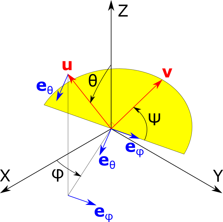
[phi, theta, psi] where phi denotes the azimuth angle from X axis to the first direction (u), theta is the latitude angle from Z axis (theta==0 -> u = Z axis), and psi is the angle defining the orientation of the second direction (v) in the plane orthogonal to u, as illustrated below:

degreesbool, default False

If True, the angles are given in degrees instead of radians.

Returns:

• float or np.ndarray – If only one direction is given as a tuple of floats [nx, ny, nz], the result is a float;

• otherwise, the result is a nd.array.

See also

eval

evaluate the function along two orthogonal directions (u,v))

mean(method='Monte Carlo', n_evals=10000, seed=None)

Estimate the mean value along all directions in the 3D space.

Parameters:

• method (str {'exact', 'Monte Carlo'}) – If ‘exact’, the full integration is performed over the unit sphere (see Notes). If method==’Monte Carlo’, the function is evaluated along a finite set of random directions. The Monte Carlo method is usually very fast, compared to the exact method.

• n_evals (int, default 10000) – If method==’Monte Carlo’, sets the number of random directions to use.

• seed (int, default None) – Sets the seed for random sampling when using the Monte Carlo method. Useful when one wants to reproduce results.

Returns:

Mean value

Return type:

float

See also

std

Standard deviation of the spherical function over the unit sphere.

Notes

The full integration over the unit sphere, used if method==’exact’, takes advantage of numpy.integrate.dblquad. This algorithm is robust but usually slow. The Monte Carlo method can be 1000 times faster.

name = 'Hyperspherical function'

Bounds to consider in spherical coordinates

plot3D(n_phi=50, n_theta=50, n_psi=50, which='mean', **kwargs)

3D plotting of a spherical function

Parameters:

• n_phi (int, default 50) – Number of azimuth angles (phi) to use for plotting. Default is 50.

• n_theta (int, default 50) – Number of latitude angles (theta) to use for plotting. Default is 50.

• n_psi (int, default 50) – Number of psi value to look for min/max/mean value (see below). Default is 50.

• which (str {'mean', 'std', 'min', 'max'}, default 'mean') – How to handle the 3rd coordinate. For instance, if which==’mean’ (default), for a given value of angles (phi, theta), the mean function value over all psi angles is plotted.

• **kwargs – These arguments will be passed to ax.plot_surface() function.

Returns:

• matplotlib.figure.Figure – Handle to the figure

• matplotlib.Axes3D – Handle to axes

See also

plot_xyz_sections

plot statistics in X-Y, X-Z and Y-Z planes

plot_xyz_sections(n_theta=500, n_psi=100)

Plot statistics in X-Y, X-Z and Y-Z planes.

The function value will be plotted as functions of the first direction (u), whereas the second direction (v) will be used to evaluate the statistics (min/max and mean).

Parameters:

• n_theta (int, default 500) – Number of values of polar angle to use for plotting

• n_psi (int, default 100) – Number of psi value to use for evaluating the statistics (mean, min and max)

Returns:

• matplotlib.figure.Figure – Handle to the figure

• matplotlib.Axes3D – Handle to axes

See also

plot3D

plot a given statistic as a 3D surface

var(method='Monte Carlo', n_evals=10000, mean=None, seed=None)

Estimate the variance along all directions in the 3D space

Parameters:

• method (str {'exact', 'Monte Carlo'}) – If ‘exact’, the full integration is performed over the unit sphere (see Notes). If method==’Monte Carlo’, the function is evaluated along a finite set of random directions. The Monte Carlo method is usually very fast, compared to the exact method.

• n_evals (int, default 10000) – If method==’Monte Carlo’, sets the number of random directions to use.

• mean (float, default None) – If provided, and if method==’exact’, skip estimation of mean value and use that provided instead.

• seed (int, default None) – Sets the seed for random sampling when using the Monte Carlo method. Useful when one wants to reproduce results.

Returns:

Variance of the function

Return type:

float

See also

mean

mean value of the function over the unit sphere.

Notes

The full integration over the unit sphere, used if method==’exact’, takes advantage of numpy.integrate.dblquad. This algorithm is robust but usually slow. The Monte Carlo method can be 1000 times faster.

class Elasticipy.SphericalFunction.SphericalFunction(fun)

Bases: object

Class for spherical functions, that is, functions that depend on directions in 3D space.

Attribute

fun : function to use

domain = array([[0.        , 6.28318531],        [0.        , 1.57079633]])

eval(u)

Evaluate value along a given (set of) direction(s).

Parameters:

u (np.ndarray or list) – Direction(s) to estimate the value along with. It can be of a unique direction [nx, ny, nz], or a set of directions (e.g. [[n1x, n1y n1z],[n2x, n2y, n2z],…]).

Returns:

If only one direction is given as a tuple of floats [nx, ny, nz], the result is a float; otherwise, the result is a nd.array.

Return type:

float or np.ndarray

See also

eval_spherical

evaluate the function along a given direction given using the spherical coordinates

eval_spherical(*args, degrees=False)

Evaluate value along a given (set of) direction(s) defined by its (their) spherical coordinates.

Parameters:

• args (list or np.ndarray) – [phi, theta] where phi denotes the azimuth angle from X axis, and theta is the latitude angle from Z axis (theta==0 -> Z axis).

• degrees (bool, default False) – If True, the angles are given in degrees instead of radians.

Returns:

If only one direction is given as a tuple of floats [phi, theta], the result is a float; otherwise, the result is a nd.array.

Return type:

float or np.ndarray

See also

eval

evaluate the function along a direction given by its cartesian coordinates

max()

Find maximum value of the function.

Returns:

• min (float) – Maximum value

• direction (np.ndarray) – direction along which the maximum value is reached

See also

min

return the minimum value and the location where it is reached

mean(method='exact', n_evals=10000, seed=None)

Estimate the mean value along all directions in the 3D space.

Parameters:

• method (str {'exact', 'Monte Carlo'}) – If ‘exact’, the full integration is performed over the unit sphere (see Notes). If method==’Monte Carlo’, the function is evaluated along a finite set of random directions. The Monte Carlo method is usually very fast, compared to the exact method.

• n_evals (int, default 10000) – If method==’Monte Carlo’, sets the number of random directions to use.

• seed (int, default None) – Sets the seed for random sampling when using the Monte Carlo method. Useful when one wants to reproduce results.

Returns:

Mean value

Return type:

float

See also

std

Standard deviation of the spherical function over the unit sphere.

Notes

The full integration over the unit sphere, used if method==’exact’, takes advantage of numpy.integrate.dblquad. This algorithm is robust but usually slow. The Monte Carlo method can be 1000 times faster.

min()

Find minimum value of the function.

Returns:

• fmin (float) – Minimum value

• dir (np.ndarray) – Direction along which the minimum value is reached

See also

max

return the maximum value and the location where it is reached

name = 'Spherical function'

Bounds to consider in spherical coordinates

plot3D(n_phi=50, n_theta=50, **kwargs)

3D plotting of a spherical function

Parameters:

• n_phi (int, default 50) – Number of azimuth angles (phi) to use for plotting. Default is 50.

• n_theta (int, default 50) – Number of latitude angles (theta) to use for plotting. Default is 50.

• **kwargs – These parameters will be passed to matplotlib plot_surface() function.

Returns:

• matplotlib.figure.Figure – Handle to the figure

• matplotlib.Axes3D – Handle to axes

See also

plot_xyz_sections

plot values of the function in X-Y, X-Z an Y-Z planes.

plot_xyz_sections(n_theta=500)

Plot values in X-Y, X-Z and Y-Z planes

Parameters:

n_theta (int, default 500) – Number of values of polar angle to use for plotting

Returns:

• matplotlib.figure.Figure – Handle to the figure

• matplotlib.Axes3D – Handle to axes

See also

plot3D

plot the values of the function over the whole unit sphere as a 3D surface

std(**kwargs)

Standard deviation of the function along all directions in the 3D space.

Parameters:

**kwargs – These parameters will be passed to var() function

Returns:

Standard deviation

Return type:

float

See also

var

variance of the function

var(method='exact', n_evals=10000, mean=None, seed=None)

Estimate the variance along all directions in the 3D space

Parameters:

• method (str {'exact', 'Monte Carlo'}) – If ‘exact’, the full integration is performed over the unit sphere (see Notes). If method==’Monte Carlo’, the function is evaluated along a finite set of random directions. The Monte Carlo method is usually very fast, compared to the exact method.

• n_evals (int, default 10000) – If method==’Monte Carlo’, sets the number of random directions to use.

• mean (float, default None) – If provided, and if method==’exact’, skip estimation of mean value and use that provided instead.

• seed (int, default None) – Sets the seed for random sampling when using the Monte Carlo method. Useful when one wants to reproduce results.

Returns:

Variance of the function

Return type:

float

See also

mean

mean value of the function over the unit sphere.

Notes

The full integration over the unit sphere, used if method==’exact’, takes advantage of numpy.integrate.dblquad. This algorithm is robust but usually slow. The Monte Carlo method can be 1000 times faster.

Elasticipy.SphericalFunction.sph2cart(*args)

Converts spherical/hyperspherical coordinates to cartesian coordinates.

Parameters:

args (tuple) – (phi, theta) angles for spherical coordinates of direction u, where phi denotes the azimuth from X and theta is the colatitude angle from Z. If a third argument is passed, it defines the third angle in hyperspherical coordinate system, that is the orientation of the second vector v, orthogonal to u.

Returns:

• np.ndarray – directions u expressed in cartesian coordinates system.

• tuple of (np.ndarray, np.ndarray) – direction of the second vector, orthogonal to u, expressed in cartesian coordinates system.

Elasticipy.SphericalFunction.uniform_spherical_distribution(n_evals, seed=None, return_orthogonal=False)

Create a set of vectors whose projections over the unit sphere are uniformly distributed.

Parameters:

• n_evals (int) – Number of vectors to generate

• seed (int, default None) – Sets the seed for the random values. Useful if one wants to ensure reproducibility.

• return_orthogonal (bool, default False) – If true, also return a second set of vectors which are orthogonal to the first one.

Returns:

• u (np.ndarray) – Random set of vectors whose projections over the unit sphere are uniform.

• v (np.ndarray) – Set of vectors with the same properties as u, but orthogonal to u. Returned only if return_orthogonal is True

Notes

The returned vector(s) are not unit. If needed, one can use:

u = (u.T / np.linalg.norm(u, axis=1)).T