Computing and plotting engineering constants
This page illustrates how one can create stiffness (or compliance) tensors, manipulate them and plot some elasticity-related values (e.g. Young modulus).
The isotropic case
As an introduction, we consider the simple case of isotropic elastic behaviour. The stiffness tensor can be constructed as follows:
>>> from elasticipy.tensors.elasticity import StiffnessTensor
>>> C = StiffnessTensor.isotropic(E=210e3, nu=0.25)
>>> print(C)
Stiffness tensor (in Voigt mapping):
[[252000.  84000.  84000.      0.      0.      0.]
 [ 84000. 252000.  84000.      0.      0.      0.]
 [ 84000.  84000. 252000.      0.      0.      0.]
 [     0.      0.      0.  84000.      0.      0.]
 [     0.      0.      0.      0.  84000.      0.]
 [     0.      0.      0.      0.      0.  84000.]]
Here, we have constructed the stiffness tensor from Young modulus and Poisson ratio. Actually, for the isotropic case, it can be constructed from any pair-values amongst the following:
Young modulus (
E),Poisson ratio,
shear modulus (
Gorlame1),bulk modulus (
K),second Lame’s parameter (
lame2).
The conversion from these pair-value to stiffness components is made from the well-known conversion table. For instance, let’s compute the shear and bulk moduli
>>> C.shear_modulus
Hyperspherical function
Min=83999.99999999991, Max=84000.00000000007
>>> print(C.bulk_modulus)
140000.0
Note
The returned value for C.shear_modulus is not a float, because in general (i.e. anisotropic case), the shear
modulus is not constant over space (see below).
One can check that both approaches yield the same tensor:
>>> C2 = StiffnessTensor.isotropic(G=84e3, K=140e3)
>>> print(C2 == C)
True
Anisotropic cases
Elasticipy supports anisotropy (actually, it was meant for that…). It supports usual material symmetries, such as orthotropy and transverse-isotropy. In additions, it also supports all crystal symmetries, as listed by [Nye] and summed up below:

Patterns of stiffness and compliance tensors of crystals, depending on their symmetries [Nye].
For example, create a stiffness tensor with monoclinic symmetry:
>>> C = StiffnessTensor.monoclinic(phase_name='TiNi',
...                                C11=231, C12=127, C13=104,
...                                C22=240, C23=131, C33=175,
...                                C44=81, C55=11, C66=85,
...                                C15=-18, C25=1, C35=-3, C46=3)
and check out the Young modulus:
>>> E = C.Young_modulus
Here E is a SphericalFunction object. It means that its value depends on the considered direction. For instance,
let’s see its value along the x, y and z directions:
>>> Ex = E.eval([1,0,0])
>>> Ey = E.eval([0,1,0])
>>> Ez = E.eval([0,0,1])
>>> print((Ex, Ey, Ez))
(np.float64(124.52232440357189), np.float64(120.92120854784433), np.float64(96.13750721721384))
Note
As the components for the stiffness tensor were provided in GPa, the values for the Young modulus are given in GPa as well.
Actually, a more compact syntax, and a faster way to do that, is to use:
>>> import numpy as np
>>> print(E.eval(np.eye(3)))
[124.5223244  120.92120855  96.13750722]
To quickly see the min/max value of a SphericalFunction, just print it:
>>> print(E)
Spherical function
Min=26.28357770763925, Max=191.39659146987594
It is clear that this material is highly anisotropic. This can be evidenced by comparing the mean and the standard deviation of the Young modulus:
>>> E_mean = E.mean()
>>> E_std = E.std()
>>> print(E_std / E_mean)
0.45580071168605646
Another way to evidence anisotropy is to use the universal anisotropy factor [Ranganathan]:
>>> print(C.universal_anisotropy)
5.141009551641412
Shear moduli and Poisson ratios
The shear modulus can be computed from the stiffness tensor as well:
>>> G = C.shear_modulus
>>> print(G)
Hyperspherical function
Min=8.748742560860755, Max=86.60555127546397
Here, the shear modulus is a HyperSphericalFunction object because its value depends on two orthogonal directions
(in other words, its arguments must lie on an unit hypersphere S3).
Let’s compute its value with respect to X and Y directions:
>>> print(G.eval([1,0,0], [0,1,0]))
84.88888888888889
The previous consideration also apply for the Poisson ratio:
>>> print(C.Poisson_ratio)
Hyperspherical function
Min=-0.5501886056193297, Max=1.4394343811866284
Plotting
Spherical functions
In order to fully evidence the directional dependence of the Young moduli, we can plot them as 3D surface:
from elasticipy.tensors.elasticity import StiffnessTensor
C = StiffnessTensor.cubic(C11=186, C12=134, C44=76)
E = C.Young_modulus
fig = E.plot3D()
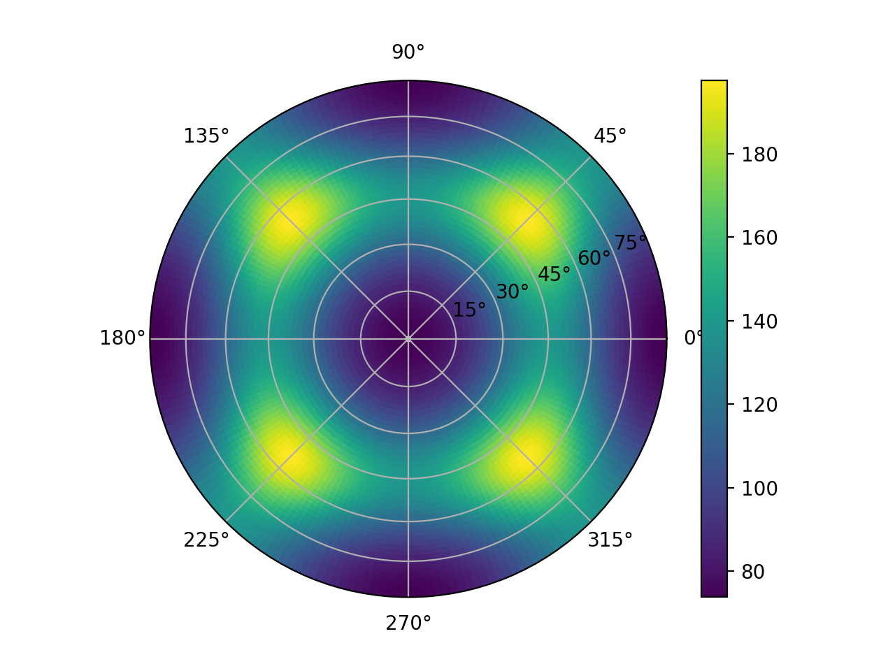
It is advised to use interactive plot to be able to zoom/rotate the surface. For flat images (i.e. to put in document/articles), we can plot the values as a Pole Figure (PF):
from elasticipy.tensors.elasticity import StiffnessTensor
C = StiffnessTensor.cubic(C11=186, C12=134, C44=77)
E = C.Young_modulus
E.plot_as_pole_figure()

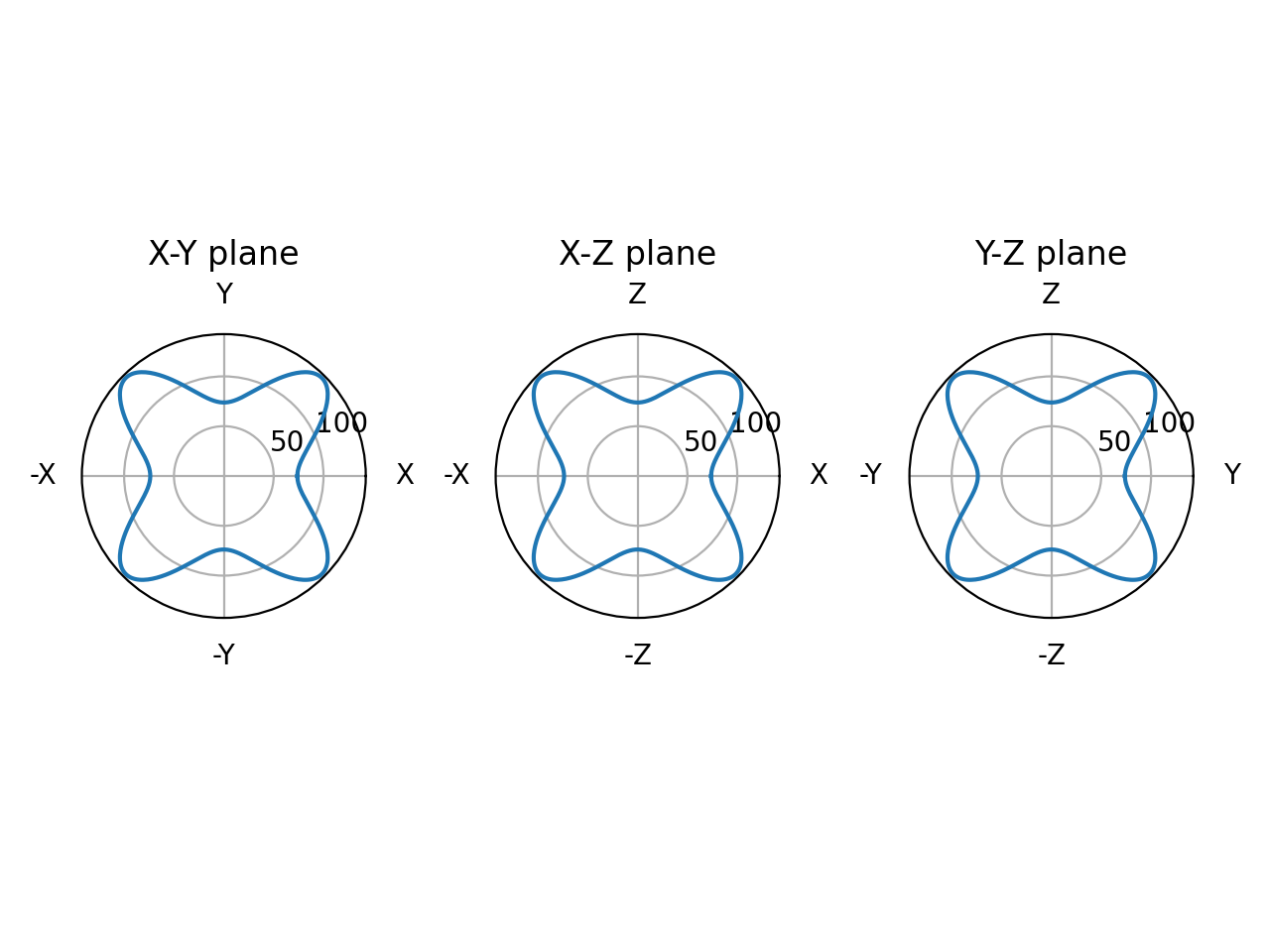
Alternatively, we can plot the Young moduli on X-Y, X-Z and Y-Z sections only:
from elasticipy.tensors.elasticity import StiffnessTensor
C = StiffnessTensor.cubic(C11=186, C12=134, C44=77)
E = C.Young_modulus
E.plot_xyz_sections()
Hyperspherical functions
Hyperspherical functions cannot plotted as 3D surfaces, as their values depend on two orthogonal directions. But at least, for a each direction u, we can consider the mean value for all the orthogonal directions v when plotting:
from elasticipy.tensors.elasticity import StiffnessTensor
C = StiffnessTensor.cubic(C11=186, C12=134, C44=77)
G = C.shear_modulus
fig = G.plot3D()
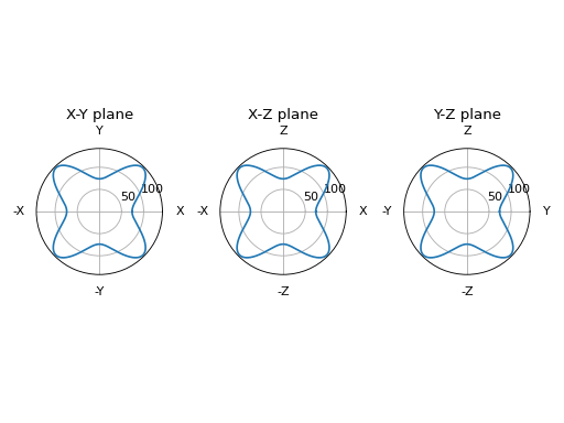
Instead of the mean value, we can consider other statistics, e.g.:
from elasticipy.tensors.elasticity import StiffnessTensor
C = StiffnessTensor.cubic(C11=186, C12=134, C44=77)
G = C.shear_modulus
fig = G.plot3D(which='min')
This also works for max and std. These parameters also apply for pole figures (see above). Actually, the min and
max values can also be plotted in the same figure, with the help of transparency:
from elasticipy.tensors.elasticity import StiffnessTensor
C = StiffnessTensor.cubic(C11=186, C12=134, C44=77)
G = C.shear_modulus
fig = G.plot3D(which='minmax')
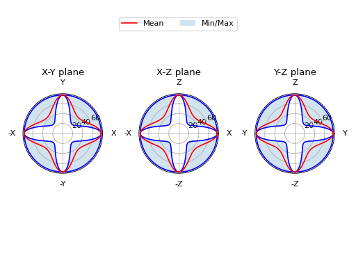
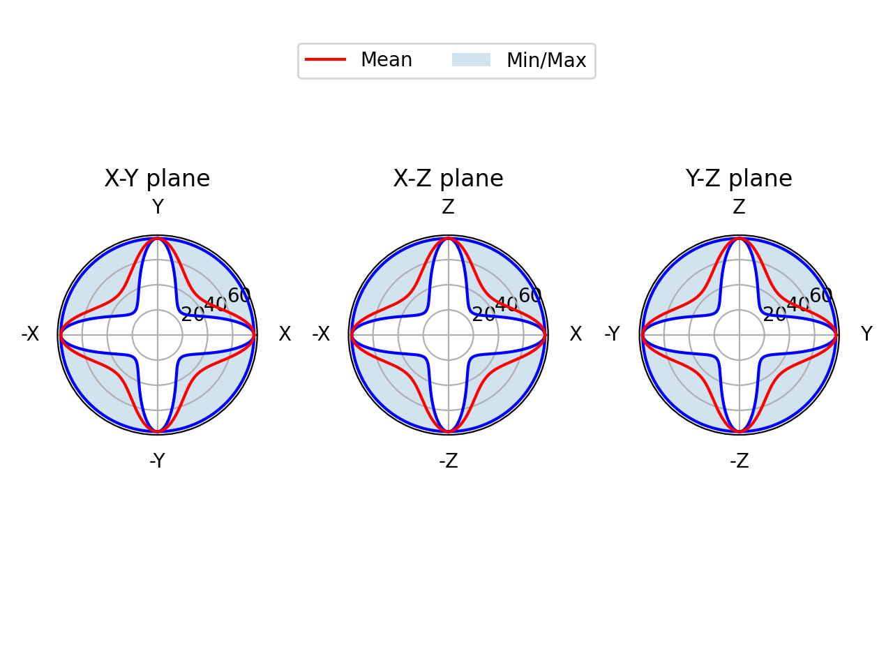
When plotting the X-Y, X-Z and Y-Z sections, the min, max and mean values are plotted at once:
from elasticipy.tensors.elasticity import StiffnessTensor
C = StiffnessTensor.cubic(C11=186, C12=134, C44=77)
G = C.shear_modulus
G.plot_xyz_sections()

Note
If you want to perform all the above tasks in a more interactive way, check out the GUI!
S. I. Ranganathan and M. Ostoja-Starzewski (2008), Universal Elastic Anisotropy Index, Phys. Rev. Lett., 101(5), 055504, . https://doi.org/10.1103/PhysRevLett.101.055504