Elasticipy.SphericalFunction module

class Elasticipy.SphericalFunction.HyperSphericalFunction(fun)

Bases: SphericalFunction

Class for defining functions that depend on two orthogonal directions u and v.

domain = array([[0.        , 6.28318531],        [0.        , 1.57079633],        [0.        , 3.14159265]])

eval(u, *args)

Evaluate the Hyperspherical function with respect to two orthogonal directions.

Parameters:

• u (list or np.ndarray) – First axis

• args (list or np.ndarray) – Second axis

Returns:

Function value

Return type:

float or np.ndarray

See also

eval_spherical

evaluate the function along a direction defined by its spherical coordinates.

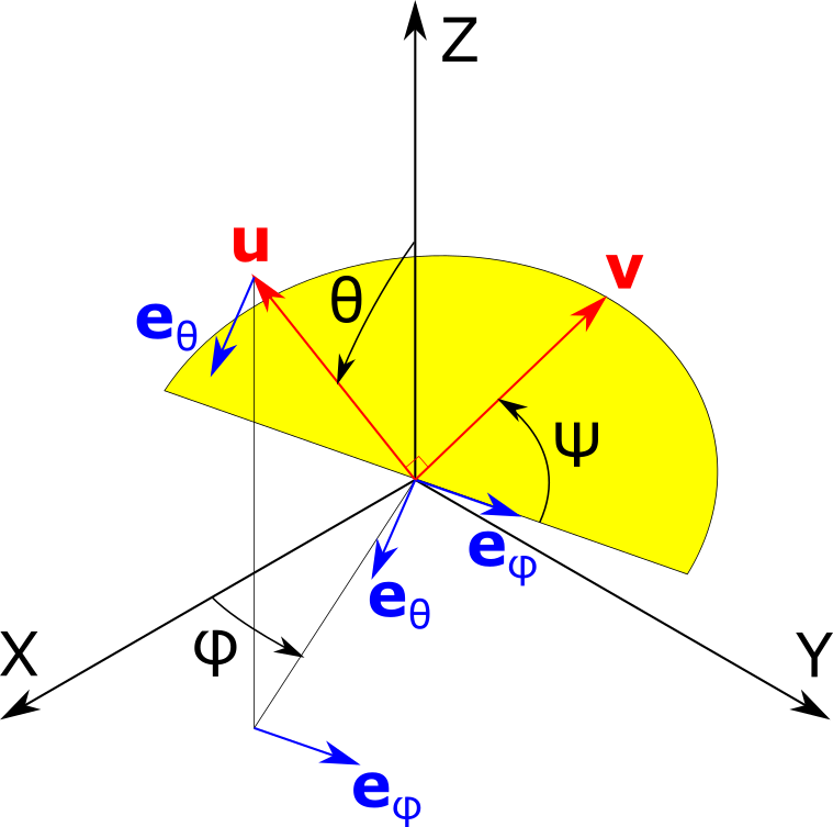
eval_spherical(*args, degrees=False)

Evaluate value along a given (set of) direction(s) defined by its (their) spherical coordinates.

Parameters:

args (list or np.ndarray) –

[phi, theta, psi] where phi denotes the azimuth angle from X axis to the first direction (u), theta is the latitude angle from Z axis (theta==0 -> u = Z axis), and psi is the angle defining the orientation of the second direction (v) in the plane orthogonal to u, as illustrated below:

degreesbool, default False

If True, the angles are given in degrees instead of radians.

Returns:

• float or np.ndarray – If only one direction is given as a tuple of floats [nx, ny, nz], the result is a float;

• otherwise, the result is a nd.array.

See also

eval

evaluate the function along two orthogonal directions (u,v))

mean(method='Monte Carlo', n_evals=10000, seed=None)

Estimate the mean value along all directions in the 3D space.

Parameters:

• method (str {'exact', 'Monte Carlo'}) – If ‘exact’, the full integration is performed over the unit sphere (see Notes). If method==’Monte Carlo’, the function is evaluated along a finite set of random directions. The Monte Carlo method is usually very fast, compared to the exact method.

• n_evals (int, default 10000) – If method==’Monte Carlo’, sets the number of random directions to use.

• seed (int, default None) – Sets the seed for random sampling when using the Monte Carlo method. Useful when one wants to reproduce results.

Returns:

Mean value

Return type:

float

See also

std

Standard deviation of the spherical function over the unit sphere.

Notes

The full integration over the unit sphere, used if method==’exact’, takes advantage of numpy.integrate.dblquad. This algorithm is robust but usually slow. The Monte Carlo method can be 1000 times faster.

name = 'Hyperspherical function'

Bounds to consider in spherical coordinates

plot3D(n_phi=50, n_theta=50, n_psi=50, which='mean', **kwargs)

Generate a 3D plot representing the evaluation of spherical harmonics.

This function evaluates a function over a grid defined by spherical coordinates (phi, theta, psi) and produces a 3D plot. It provides options to display the mean, standard deviation, minimum, or maximum of the evaluated values along the third angles (psi). The plot can be customized with additional keyword arguments.

Parameters:

• n_phi (int, optional) – Number of divisions along the phi axis, default is 50.

• n_theta (int, optional) – Number of divisions along the theta axis, default is 50.

• n_psi (int, optional) – Number of divisions along the psi axis, default is 50.

• which (str, optional) – Determines which statistical measure to plot (‘mean’, ‘std’, ‘min’, ‘max’), default is ‘mean’.

• kwargs (dict, optional) – Additional keyword arguments to customize the plot.

Returns:

A tuple containing the matplotlib figure and axes objects.

Return type:

tuple

plot_as_pole_figure(n_theta=50, n_phi=200, n_psi=50, which='mean', projection='lambert', fig=None, plot_type='imshow', **kwargs)

Generate a pole figure plot from spherical function evaluation.

This function evaluates a spherical function over specified ranges of angles (phi, theta, psi) and then generates a 2D pole figure plot using various statistical summaries of the data (mean, std, min, max). It also supports several types of plot visualizations such as ‘imshow’, ‘contourf’, and ‘contour’.

Parameters:

• n_theta (int, optional) – Number of sampling points for theta angle. Default is 50.

• n_phi (int, optional) – Number of sampling points for phi angle. Default is 200.

• n_psi (int, optional) – Number of sampling points for psi angle. Default is 50.

• which (str, optional) – Specifies the type of statistical summary to use for plotting. Options include ‘mean’, ‘std’, ‘min’, ‘max’. Default is ‘mean’.

• projection (str, optional) – Type of projection for the pole figure plot. Default is ‘lambert’.

• fig (matplotlib.figure.Figure, optional) – Pre-existing figure to use for plotting. If None, a new figure is created. Default is None.

• plot_type (str, optional) – Type of plot to generate. Can be ‘imshow’, ‘contourf’, or ‘contour’. Default is ‘imshow’.

• **kwargs (dict, optional) – Additional keyword arguments passed to the plotting functions.

Returns:

• fig (matplotlib.figure.Figure) – The figure object containing the plot.

• ax (matplotlib.axes.Axes) – The axes object containing the plot.

plot_xyz_sections(n_theta=500, n_psi=100, color_minmax='blue', alpha_minmax=0.2, color_mean='red')

Plots the XYZ sections using polar projections.

This function creates a figure with three subplots representing the XY, XZ, and YZ sections. It utilizes polar projections to plot the min, max, and mean values of the evaluated function over given theta and phi ranges.

Parameters:

• n_theta (int, optional) – Number of theta points to use in the grid (default is 500).

• n_psi (int, optional) – Number of psi points to use in the grid (default is 100).

• color_minmax (str, optional) – Color to use for plotting min and max values (default is ‘blue’).

• alpha_minmax (float, optional) – Alpha transparency level to use for the min/max fill (default is 0.2).

• color_mean (str, optional) – Color to use for plotting mean values (default is ‘red’).

Returns:

• fig (matplotlib.figure.Figure) – The created figure.

• axs (list of matplotlib.axes._subplots.PolarAxesSubplot) – List of polar axis subplots.

var(method='Monte Carlo', n_evals=10000, mean=None, seed=None)

Estimate the variance along all directions in the 3D space

Parameters:

• method (str {'exact', 'Monte Carlo'}) – If ‘exact’, the full integration is performed over the unit sphere (see Notes). If method==’Monte Carlo’, the function is evaluated along a finite set of random directions. The Monte Carlo method is usually very fast, compared to the exact method.

• n_evals (int, default 10000) – If method==’Monte Carlo’, sets the number of random directions to use.

• mean (float, default None) – If provided, and if method==’exact’, skip estimation of mean value and use that provided instead.

• seed (int, default None) – Sets the seed for random sampling when using the Monte Carlo method. Useful when one wants to reproduce results.

Returns:

Variance of the function

Return type:

float

See also

mean

mean value of the function over the unit sphere.

Notes

The full integration over the unit sphere, used if method==’exact’, takes advantage of numpy.integrate.dblquad. This algorithm is robust but usually slow. The Monte Carlo method can be 1000 times faster.

class Elasticipy.SphericalFunction.SphericalFunction(fun)

Bases: object

Class for spherical functions, that is, functions that depend on directions in 3D space.

Attribute

fun : function to use

domain = array([[0.        , 6.28318531],        [0.        , 1.57079633]])

eval(u)

Evaluate value along a given (set of) direction(s).

Parameters:

u (np.ndarray or list) – Direction(s) to estimate the value along with. It can be of a unique direction [nx, ny, nz], or a set of directions (e.g. [[n1x, n1y n1z],[n2x, n2y, n2z],…]).

Returns:

If only one direction is given as a tuple of floats [nx, ny, nz], the result is a float; otherwise, the result is a nd.array.

Return type:

float or np.ndarray

See also

eval_spherical

evaluate the function along a given direction given using the spherical coordinates

eval_spherical(*args, degrees=False)

Evaluate value along a given (set of) direction(s) defined by its (their) spherical coordinates.

Parameters:

• args (list or np.ndarray) – [phi, theta] where phi denotes the azimuth angle from X axis, and theta is the latitude angle from Z axis (theta==0 -> Z axis).

• degrees (bool, default False) – If True, the angles are given in degrees instead of radians.

Returns:

If only one direction is given as a tuple of floats [phi, theta], the result is a float; otherwise, the result is a nd.array.

Return type:

float or np.ndarray

See also

eval

evaluate the function along a direction given by its cartesian coordinates

max()

Find maximum value of the function.

Returns:

• min (float) – Maximum value

• direction (np.ndarray) – direction along which the maximum value is reached

See also

min

return the minimum value and the location where it is reached

mean(method='exact', n_evals=10000, seed=None)

Estimate the mean value along all directions in the 3D space.

Parameters:

• method (str {'exact', 'Monte Carlo'}) – If ‘exact’, the full integration is performed over the unit sphere (see Notes). If method==’Monte Carlo’, the function is evaluated along a finite set of random directions. The Monte Carlo method is usually very fast, compared to the exact method.

• n_evals (int, default 10000) – If method==’Monte Carlo’, sets the number of random directions to use.

• seed (int, default None) – Sets the seed for random sampling when using the Monte Carlo method. Useful when one wants to reproduce results.

Returns:

Mean value

Return type:

float

See also

std

Standard deviation of the spherical function over the unit sphere.

Notes

The full integration over the unit sphere, used if method==’exact’, takes advantage of numpy.integrate.dblquad. This algorithm is robust but usually slow. The Monte Carlo method can be 1000 times faster.

min()

Find minimum value of the function.

Returns:

• fmin (float) – Minimum value

• dir (np.ndarray) – Direction along which the minimum value is reached

See also

max

return the maximum value and the location where it is reached

name = 'Spherical function'

Bounds to consider in spherical coordinates

plot3D(n_phi=50, n_theta=50, **kwargs)

3D plotting of a spherical function

Parameters:

• n_phi (int, default 50) – Number of azimuth angles (phi) to use for plotting. Default is 50.

• n_theta (int, default 50) – Number of latitude angles (theta) to use for plotting. Default is 50.

• **kwargs – These parameters will be passed to matplotlib plot_surface() function.

Returns:

• matplotlib.figure.Figure – Handle to the figure

• matplotlib.Axes3D – Handle to axes

See also

plot_xyz_sections

plot values of the function in X-Y, X-Z an Y-Z planes.

plot_as_pole_figure(n_theta=50, n_phi=200, projection='lambert', fig=None, plot_type='imshow', **kwargs)

Plots a pole figure visualization of spherical data using specified parameters and plot types.

The function creates a pole figure based on spherical coordinates and can use different types of plots including ‘imshow’, ‘contourf’, and ‘contour’. It also supports a variety of projections and renders the figure using Matplotlib.

Parameters:

• n_theta (int, optional) – Number of divisions in the theta dimension, by default 50.

• n_phi (int, optional) – Number of divisions in the phi dimension, by default 200.

• projection (str {'Lambert','equal area'}, optional) – The type of projection to use for the plot, by default ‘Lambert’.

• fig (matplotlib.figure.Figure, optional) – A Matplotlib figure object. If None, a new figure will be created, by default None.

• plot_type (str, optional) – The type of plot to generate: ‘imshow’, ‘contourf’, or ‘contour’, by default ‘imshow’.

• **kwargs (dict) – Additional keyword arguments to pass to the plotting functions.

Returns:

• fig (matplotlib.figure.Figure) – The Matplotlib figure containing the plot.

• ax (matplotlib.axes._axes.Axes) – The Matplotlib axes of the plot.

plot_xyz_sections(n_theta=500, **kwargs)

Plot XYZ sections of spherical data.

This method generates a figure with three polar plots showing the XY, XZ, and YZ sections of the spherical data contained within the instance. Each section is plotted using n_theta evenly spaced points over the interval [0, 2π].

Parameters:

• n_theta (int, optional) – Number of points to use for the polar plot angles. Default is 500.

• **kwargs (dict, optional) – Additional keyword arguments to pass to the plot function.

Returns:

• fig (matplotlib.figure.Figure) – The figure object containing the polar plots.

• axs (list of matplotlib.axes._subplots.PolarAxesSubplot) – List of axes objects for each plot.

std(**kwargs)

Standard deviation of the function along all directions in the 3D space.

Parameters:

**kwargs – These parameters will be passed to var() function

Returns:

Standard deviation

Return type:

float

See also

var

variance of the function

var(method='exact', n_evals=10000, mean=None, seed=None)

Estimate the variance along all directions in the 3D space

Parameters:

• method (str {'exact', 'Monte Carlo'}) – If ‘exact’, the full integration is performed over the unit sphere (see Notes). If method==’Monte Carlo’, the function is evaluated along a finite set of random directions. The Monte Carlo method is usually very fast, compared to the exact method.

• n_evals (int, default 10000) – If method==’Monte Carlo’, sets the number of random directions to use.

• mean (float, default None) – If provided, and if method==’exact’, skip estimation of mean value and use that provided instead.

• seed (int, default None) – Sets the seed for random sampling when using the Monte Carlo method. Useful when one wants to reproduce results.

Returns:

Variance of the function

Return type:

float

See also

mean

mean value of the function over the unit sphere.

Notes

The full integration over the unit sphere, used if method==’exact’, takes advantage of numpy.integrate.dblquad. This algorithm is robust but usually slow. The Monte Carlo method can be 1000 times faster.

Elasticipy.SphericalFunction.sph2cart(*args)

Converts spherical/hyperspherical coordinates to cartesian coordinates.

Parameters:

args (tuple) – (phi, theta) angles for spherical coordinates of direction u, where phi denotes the azimuth from X and theta is the colatitude angle from Z. If a third argument is passed, it defines the third angle in hyperspherical coordinate system, that is the orientation of the second vector v, orthogonal to u.

Returns:

• np.ndarray – directions u expressed in cartesian coordinates system.

• tuple of (np.ndarray, np.ndarray) – direction of the second vector, orthogonal to u, expressed in cartesian coordinates system.

Elasticipy.SphericalFunction.uniform_spherical_distribution(n_evals, seed=None, return_orthogonal=False)

Create a set of vectors whose projections over the unit sphere are uniformly distributed.

Parameters:

• n_evals (int) – Number of vectors to generate

• seed (int, default None) – Sets the seed for the random values. Useful if one wants to ensure reproducibility.

• return_orthogonal (bool, default False) – If true, also return a second set of vectors which are orthogonal to the first one.

Returns:

• u (np.ndarray) – Random set of vectors whose projections over the unit sphere are uniform.

• v (np.ndarray) – Set of vectors with the same properties as u, but orthogonal to u. Returned only if return_orthogonal is True

Notes

The returned vector(s) are not unit. If needed, one can use:

u = (u.T / np.linalg.norm(u, axis=1)).T