Averaging multiple phases

In this tutorial, we will see how we can compute the lower and upper bounds of elastic properties of a two-phased material.

Example: duplex steel

We consider the duplex stainless steel. It is composed of a BCC austenitic phase, and FCC ferritic phase. The stiffness tensor of each phase are roughly:

\[\begin{split}\mathbf{C}_{aust} = \begin{bmatrix} 204 & 137 & 137 & 0 & 0 & 0\\ 137 & 204 & 137 & 0 & 0 & 0\\ 137 & 137 & 204 & 0 & 0 & 0\\ 0 & 0 & 0 & 126 & 0 & 0\\ 0 & 0 & 0 & 0 & 126 & 0\\ 0 & 0 & 0 & 0 & 0 & 126 \end{bmatrix}\end{split}\]

\[\begin{split}\mathbf{C}_{ferr} = \begin{bmatrix} 242 & 146 & 146 & 0 & 0 & 0\\ 137 & 242 & 146 & 0 & 0 & 0\\ 137 & 137 & 242 & 0 & 0 & 0\\ 0 & 0 & 0 & 116 & 0 & 0\\ 0 & 0 & 0 & 0 & 116 & 0\\ 0 & 0 & 0 & 0 & 0 & 116 \end{bmatrix}\end{split}\]

Voigt and Reuss averages

Let’s start by creating the two stiffness tensors in Python:

>>> from Elasticipy.FourthOrderTensor import StiffnessTensor
>>> C_austenite = StiffnessTensor.cubic(C11=204, C12=137, C44=126)
>>> C_ferrite = StiffnessTensor.cubic(C11=242, C12=146, C44=116)

Lower bounds of elastic moduli

The lower bound of elastic moduli is given by the Reuss averages of stiffness tensors. Assuming that neither the austenite nor the ferrite phased have remarkable crystallographic texture, we can compute the resulting isotropic stiffness tensor for each phase:

>>> C_austenite_ravg = C_austenite.Reuss_average()
>>> C_ferrite_ravg = C_ferrite.Reuss_average()

Finally, the lower bound for the stiffness tensor of the duplex steel is given by the Reuss average of the both the aforementioned tensors, weighted by the volume fraction of each phase (say, 40/60 here):

>>> C_reuss = StiffnessTensor.weighted_average((C_austenite_ravg, C_ferrite_ravg), (0.4, 0.6), 'Reuss')

Now we can check out the lower bound for the Young modulus:

>>> print(C_reuss.Young_modulus.mean())
179.16068408455897

Upper bound of elastic moduli

Conversely, the upper bounds of elastic moduli is given by the Voigt averages. The commands above become:

>>> C_austenite_vavg = C_austenite.Hill_average()
>>> C_ferrite_vavg = C_ferrite.Hill_average()
>>> C_voigt = StiffnessTensor.weighted_average((C_austenite_vavg, C_ferrite_vavg), (0.4, 0.6), 'Voigt')

Which leads to:

>>> print(C_voigt.Young_modulus.mean())
204.45867599496472

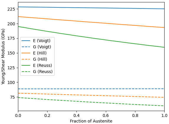
Plotting the averages as functions of the volume fraction

In order to investigate the influence of austenite volume fraction on the elastic moduli, one can use the following commands:

>>> import numpy as np
>>> from matplotlib import pyplot as plt
>>> n_values = 100
>>> fraction_austenite = np.linspace(0, 1, n_values)
>>> fig, ax = plt.subplots()
>>> colors = plt.cm.tab10.colors    # Simple hack to ensure that both E and G will have the same color for a given method
>>> color_index = 0
>>> for method in ('Voigt', 'Hill', 'Reuss'):
>>>     C_aust_avg = C_austenite.average(method)    # Equivalent to C_austenite.{method}_average()
>>>     C_ferr_avg = C_ferrite.average(method)
>>>     E_mean = np.zeros(n_values)
>>>     G_mean = np.zeros(n_values)
>>>     for i in range(n_values):
>>>         f1 = fraction_austenite[i]
>>>         f2 = 1 - f1
>>>         C_tot_mean = StiffnessTensor.weighted_average((C_aust_avg, C_ferr_avg), (f1, f2), method)
>>>         E_mean[i] = C_tot_mean.Young_modulus.mean()
>>>         G_mean[i] = C_tot_mean.shear_modulus.mean()
>>>     ax.plot(fraction_austenite, E_mean, label='E ({})'.format(method), color=colors[color_index])
>>>     ax.plot(fraction_austenite, G_mean, label='G ({})'.format(method), color=colors[color_index], linestyle='--')
>>>     color_index = color_index + 1
>>> ax.legend()
>>> ax.set_xlim([0, 1])
>>> ax.set_xlabel('Fraction of Austenite')
>>> ax.set_ylabel('Young/Shear Modulus (GPa)')
>>> fig.show()

leading to: