Computing wave velocities
In this tutorial, we will see how one can compute the wave velocities in an (an)isotropic material, given its stiffness tensor and its mass density.
Creating the p- and s-wave velocity functions
We will try to replicate the great tutorial made for MTEX user available here. We thus start by defining the stiffness tensor for forsterite:
>>> from Elasticipy.FourthOrderTensor import StiffnessTensor
>>> C = StiffnessTensor.orthorhombic(phase_name='forsterite',
...                                  C11=320, C12=68.2, C13=71.6, C22=196.5, C23=76.8,
...                                  C33=233.5, C44=64, C55=77, C66=78.7)
>>> print(C)
Stiffness tensor (in Voigt notation) for forsterite:
[[320.   68.2  71.6   0.    0.    0. ]
 [ 68.2 196.5  76.8   0.    0.    0. ]
 [ 71.6  76.8 233.5   0.    0.    0. ]
 [  0.    0.    0.   64.    0.    0. ]
 [  0.    0.    0.    0.   77.    0. ]
 [  0.    0.    0.    0.    0.   78.7]]
Symmetry: orthorhombic
And define the mass density:
>>> rho = 3.36
Note
You should be careful about the unit you use. Since our stiffness is given in GPa, we have to use rho in kg/dm³
in order to get the velocities in km/s. Look at the full documentation for details.
Now, we can define 3 spherical functions, which correspond to velocities of:
the compressive wave (a.k.a the primary wave);
the fast shear wave (a.k.a. the fast secondary wave);
the slow shear wave (a.k.a. the slow secondary wave);
>>> cp, cs_fast, cs_slow = C.wave_velocity(rho)
One can check that for a given direction (say, x)
>>> x = [1, 0, 0]
>>> print(cp.eval(x), cs_fast.eval(x), cs_slow.eval(x))
9.759000729485331 4.839692040576451 4.7871355387816905
Plotting the wave velocities
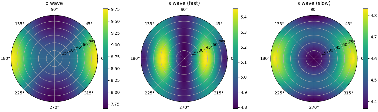
Now, we can plot all the velocities on three independent pole figures:
>>> fig, _ = cp.plot_as_pole_figure(subplot_args=(131,), title='p wave', show=False)
>>> cs_fast.plot_as_pole_figure(subplot_args=(132,), title='s wave (fast)', fig=fig, show=False)
>>> cs_slow.plot_as_pole_figure(subplot_args=(133,), title='s wave (slow)', fig=fig, show=True)
Note
We pass subplot_args to create the subplots. The option show=false temporary disables showing the figure;
this is necessary here to be plot multiple figures at once.
For further details about plotting options, see here.