Plasticity

Although Elasticipy was not initially meant to work on plasticity (hence the name…), it provides some clues about simulations of elasto-plastic behaviour of materials. This tutorial shows how one can simulate a tensile test in the elasto-plastic domain of a material.

The Johnson-Cook model

The Johnson-Cook (JC) model is widely used in the literature for modeling isotropic hardening of metalic materials. Therefore, it is available out-of-the-box in Elasticipy. It assumes that the flow stress (\(\sigma\)) depends on the equivalent strain (\(\varepsilon\)), the strain rate (\(\dot{\varepsilon}\)) and the temperature (\(T\)), according to the following equation:

\[\sigma = \left(A + B\varepsilon^n\right) \left[1 + C\log\left(\frac{\varepsilon}{\dot{\varepsilon}_0}\right)\right] \left(1-\theta^m\right)\]

with

\[\begin{split}\theta = \begin{cases} \frac{T-T_0}{T_m-T_0} & \text{if } T<T_m\\\\ 1 & \text{otherwise} \end{cases}\end{split}\]

\(A\), \(B\), \(C\), \(\dot{\varepsilon}_0\), \(T_0\), \(T_m\) and \(m\) are parameters whose values depend on the material.

Simulation of a stress-controlled tensile test

At first, we will try to simulate a stress-controlled tensile test. Although this approach is quite uncommon, we will do this anyway, just because it is easier to program.

First, let us create the model:

>>> from Elasticipy.plasticity import JohnsonCook
>>> JC = JohnsonCook(A=363, B=792.7122, n=0.5756)

The parameters are taken from [1]. As we will also take elastic behaviour into account, we also need:

>>> from Elasticipy.tensors.elasticity import StiffnessTensor
>>> C = StiffnessTensor.isotropic(E=210000, nu=0.27)

Now, let say that we want to investigate the material’s response for the tensile stress ranging from 0 to 725 MPa:

>>> from Elasticipy.tensors.stress_strain import StressTensor, StrainTensor
>>> import numpy as np
>>> n_step = 100
>>> stress_mag = np.linspace(0, 725, n_step)
>>> stress = StressTensor.tensile([1,0,0], stress_mag)

At least, we can directly compute the elastic strain for each step:

>>> elastic_strain = C.inv() * stress

So now, the plastic strain can be computed using an iterative approach:

>>> plastic_strain = StrainTensor.zeros(n_step)
>>> for i in range(1, n_step):
...       strain_increment = JC.compute_strain_increment(stress[i])
...       plastic_strain[i] = plastic_strain[i-1] + strain_increment

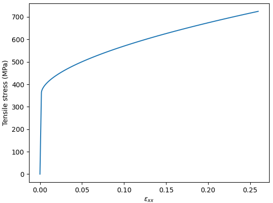
That’s all. Finally, let us plot the applied stress as a function of the overall elongation:

>>> from matplotlib import pyplot as plt
>>> elong = elastic_strain.C[0,0]+plastic_strain.C[0,0]
>>> fig, ax = plt.subplots()
>>> ax.plot(elong, stress_mag, label='Stress-controlled')
>>> ax.set_xlabel(r'$\varepsilon_{xx}$')
>>> ax.set_ylabel('Tensile stress (MPa)')

Now, let say that we want to investigate the material’s response for the tensile stress ranging from 0 to 725 MPa:

>>> import numpy as np
>>> n_step = 100
>>> stress_mag = np.linspace(0, 725, n_step)
>>> stress = StressTensor.tensile([1,0,0], stress_mag)

At least, we can directly compute the elastic strain for each step:

>>> elastic_strain = C.inv() * stress

So now, the plastic strain can be computed using an iterative approach:

>>> plastic_strain = StrainTensor.zeros(n_step)
>>> for i in range(1, n_step):
...       strain_increment = JC.compute_strain_increment(stress[i])
...       plastic_strain[i] = plastic_strain[i-1] + strain_increment

That’s all. Finally, let us plot the applied stress as a function of the overall elongation:

>>> from matplotlib import pyplot as plt
>>> elong = elastic_strain.C[0,0]+plastic_strain.C[0,0]
>>> fig, ax = plt.subplots()
>>> ax.plot(elong, stress_mag, label='Stress-controlled')
>>> ax.set_xlabel(r'$\varepsilon_{xx}$')
>>> ax.set_ylabel('Tensile stress (MPa)')

Simulation of a strain-controlled tensile test

The difficulty of simulating a strain-controlled tensile test is that, at a given step, one must identify both the elastic and the plastic strain (if any) at once, while ensuring that the stress keeps uniaxial. Therefore, the hack is to add a subroutine (optimization loop) to find the tensile stress so that the associated strain complies with the applied strain:

>>> from scipy.optimize import minimize_scalar
>>> JC.reset_strain() # Ensure that the previous hardening does not count
>>> stress = StressTensor.zeros(n_step)
>>> plastic_strain = StrainTensor.zeros(n_step)
>>> JC.reset_strain()
>>> for i in range(1, n_step):
...        def fun(tensile_stress):
...            trial_stress = StressTensor.tensile([1,0,0], tensile_stress)
...            trial_elastic_strain = C.inv() * trial_stress
...            trial_strain_increment = JC.compute_strain_increment(trial_stress, apply_strain=False)
...            trial_plastic_strain = plastic_strain[i - 1] + trial_strain_increment
...            trial_elongation =  trial_plastic_strain.C[0,0] +  trial_elastic_strain.C[0,0]
...            return (trial_elongation - elong[i])**2
...        s = minimize_scalar(fun)
...        stress.C[0,0][i] = s.x
...        strain_increment = JC.compute_strain_increment(stress[i])
...        plastic_strain[i] = plastic_strain[i-1] + strain_increment

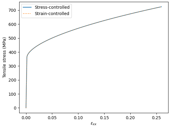
Finally, let’s plot the corresponding tensile curve ontop of that of the stress-controlled tensile test:

>>> ax.plot(elong, stress.C[0,0], label='Strain-controlled', linestyle='dotted')
>>> ax.legend()

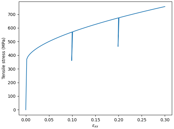
Incremental loading

Here, we have only considered monotonic loading, but we can also consider different loading path, such as incremental:

>>> load_path = [np.linspace(0,0.1),
...              np.linspace(0.1,0.099),
...              np.linspace(0.099,0.2),
...              np.linspace(0.2,0.199),
...              np.linspace(0.199,0.3)]
>>> elong = np.concatenate(load_path)
>>> n_step = len(elong)

or cyclic:

>>> load_path = [np.linspace(0,0.1),
...              np.linspace(0.1,-0.2),
...              np.linspace(-0.2,0.3),
...              np.linspace(0.3,-0.4)]
>>> elong = np.concatenate(load_path)
>>> n_step = len(elong)

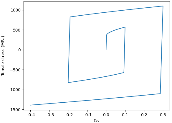
Note

The figure above clearly evidences the isotropic hardening inherent to the JC model.

Complex loading path

In the example above, we have only studied longitudinal stress/strain. Still, it is worth mentioning that other stress states can be investigated (e.g. shear, multiaxial etc.) thanks to the normality rule.

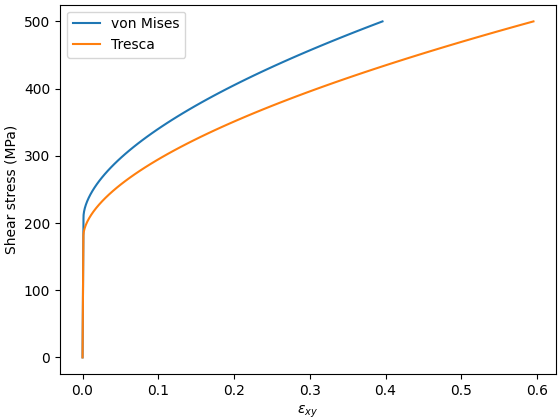
Tresca’s plasticity criterion

Above, we have used the von Mises plasticity criterion (a.k.a J2 criterion). This can be switched to Tresca by passing the plasticity criterion to the model constructor:

>>> JC = JohnsonCook(A=363, B=792.7122, n=0.5756, criterion='Tresca')

For instance, one can highlight the difference between the J2 and Tresca plasticity in shear:

>>> JC.reset_strain()
>>> JC_tresca = JohnsonCook(A=363, B=792.7122, n=0.5756, criterion='Tresca')
>>> stress_mag = np.linspace(0, 500, n_step)
>>> stress = StressTensor.shear([1,0,0], [0,1,0],stress_mag)
>>> models = (JC, JC_tresca)
>>> labels = ('von Mises', 'Tresca')
>>>
>>> elastic_strain = C.inv() * stress
>>> fig, ax = plt.subplots()
>>> for j, model in enumerate(models):
    ... plastic_strain = StrainTensor.zeros(n_step)
    ... for i in range(1, n_step):
    ...     strain_increment = model.compute_strain_increment(stress[i])
    ...     plastic_strain[i] = plastic_strain[i-1] + strain_increment
    ... eps_xy = elastic_strain.C[0,1]+plastic_strain.C[0,1]
    ... ax.plot(eps_xy, stress_mag, label=labels[j])
>>> ax.set_xlabel(r'$\varepsilon_{xy}$')
>>> ax.set_ylabel('Shear stress (MPa)')
>>> ax.legend()

[1]

Sandeep Yadav, Sorabh Singhal, Yogeshwar Jasra, Ravindra K. Saxena, Determination of Johnson-Cook material model for weldment of mild steel, Materials Today: Proceedings, Volume 28, Part 3, 2020, Pages 1801-1808, ISSN 2214-7853, https://doi.org/10.1016/j.matpr.2020.05.213.