Computing and plotting engineering constants
This page illustrates how one can create stiffness (or compliance) tensors, manipulate them and plot some elasticity-related values (e.g. Young modulus).
The isotropic case
As an introduction, we consider the simple case of isotropic elastic behaviour. The stiffness tensor can be constructed as follows:
>>> from elasticipy.tensors.elasticity import StiffnessTensor
>>> C = StiffnessTensor.isotropic(E=210e3, nu=0.25)
>>> print(C)
Stiffness tensor (in Voigt mapping):
[[252000.  84000.  84000.      0.      0.      0.]
 [ 84000. 252000.  84000.      0.      0.      0.]
 [ 84000.  84000. 252000.      0.      0.      0.]
 [     0.      0.      0.  84000.      0.      0.]
 [     0.      0.      0.      0.  84000.      0.]
 [     0.      0.      0.      0.      0.  84000.]]
Here, we have constructed the stiffness tensor from Young modulus and Poisson ratio. Actually, for the isotropic case, it can be constructed from any pair-values amongst the following:
Young modulus (
E),Poisson ratio,
shear modulus (
Gorlame1),bulk modulus (
K),second Lame’s parameter (
lame2).
The conversion from these pair-value to stiffness components is made from the well-known conversion table. For instance, let’s compute the shear and bulk moduli
>>> C.shear_modulus
Hyperspherical function
Min=83999.99999999991, Max=84000.00000000007
>>> C.bulk_modulus
140000.0
Note
The returned value for C.shear_modulus is not a float, because in general (i.e. anisotropic case), the shear
modulus is not constant over space (see below).
One can check that both approaches yield the same tensor:
>>> C2 = StiffnessTensor.isotropic(G=84e3, K=140e3)
>>> C2 == C
True
Anisotropic cases
Elasticipy supports anisotropy (actually, it was meant for that…). It supports usual material symmetries, such as orthotropy and transverse-isotropy. In additions, it also supports all crystal symmetries, as listed by [Nye] and summed up below:
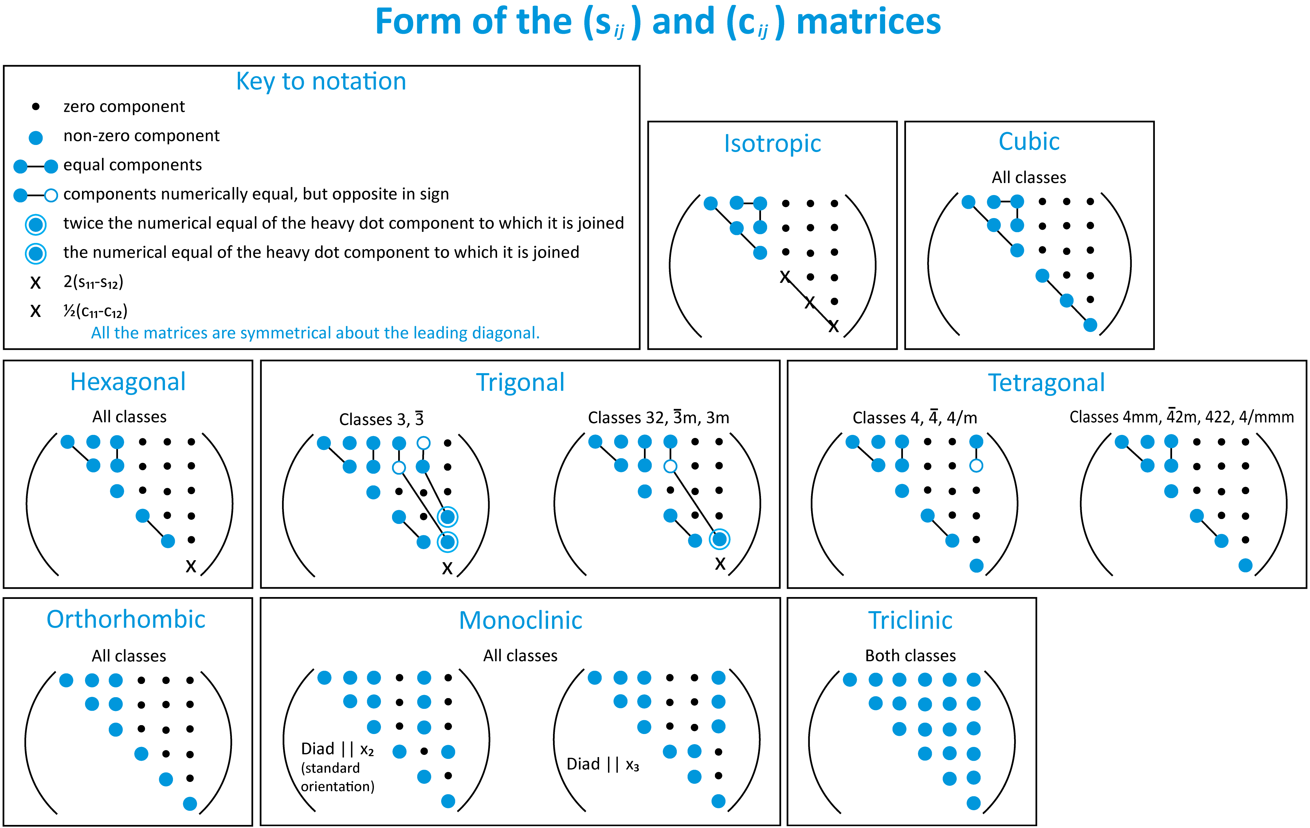
Patterns of stiffness and compliance tensors of crystals, depending on their symmetries [Nye].
For example, create a stiffness tensor with monoclinic symmetry:
>>> C = StiffnessTensor.monoclinic(phase_name='TiNi',
...                                C11=231, C12=127, C13=104,
...                                C22=240, C23=131, C33=175,
...                                C44=81, C55=11, C66=85,
...                                C15=-18, C25=1, C35=-3, C46=3)
and check out the Young modulus:
>>> E = C.Young_modulus
Here E is a SphericalFunction object. It means that its value depends on the considered direction. For instance,
let’s see its value along the x, y and z directions:
>>> Ex = E.eval([1,0,0])
>>> Ey = E.eval([0,1,0])
>>> Ez = E.eval([0,0,1])
>>> print((Ex, Ey, Ez))
(124.52232440357189, 120.92120854784433, 96.13750721721384)
Note
As the components for the stiffness tensor were provided in GPa, the values for the Young modulus are given in GPa as well.
Actually, a more compact syntax, and a faster way to do that, is to use:
>>> import numpy as np
>>> print(E.eval(np.eye(3)))
[124.5223244  120.92120855  96.13750722]
To quickly see the min/max value of a SphericalFunction, just print it:
>>> print(E)
Spherical function
Min=26.28357770763925, Max=191.39659146987594
It is clear that this material is highly anisotropic. This can be evidenced by comparing the mean and the standard deviation of the Young modulus:
>>> E_mean = E.mean()
>>> E_std = E.std()
>>> print(E_std / E_mean)
0.45580071168605646
Another way to evidence anisotropy is to use the universal anisotropy factor [Ranganathan]:
>>> C.universal_anisotropy
5.141009551641412
Shear moduli and Poisson ratios
The shear modulus can be computed from the stiffness tensor as well:
>>> G = C.shear_modulus
>>> print(G)
Hyperspherical function
Min=8.748742560860755, Max=86.60555127546397
Here, the shear modulus is a HyperSphericalFunction object because its value depends on two orthogonal directions
(in other words, its arguments must lie on an unit hypersphere S3).
Let’s compute its value with respect to X and Y directions:
>>> print(G.eval([1,0,0], [0,1,0]))
84.88888888888889
The previous consideration also apply for the Poisson ratio:
>>> print(C.Poisson_ratio)
Hyperspherical function
Min=-0.5501886056193297, Max=1.4394343811866284
Plotting
Spherical functions
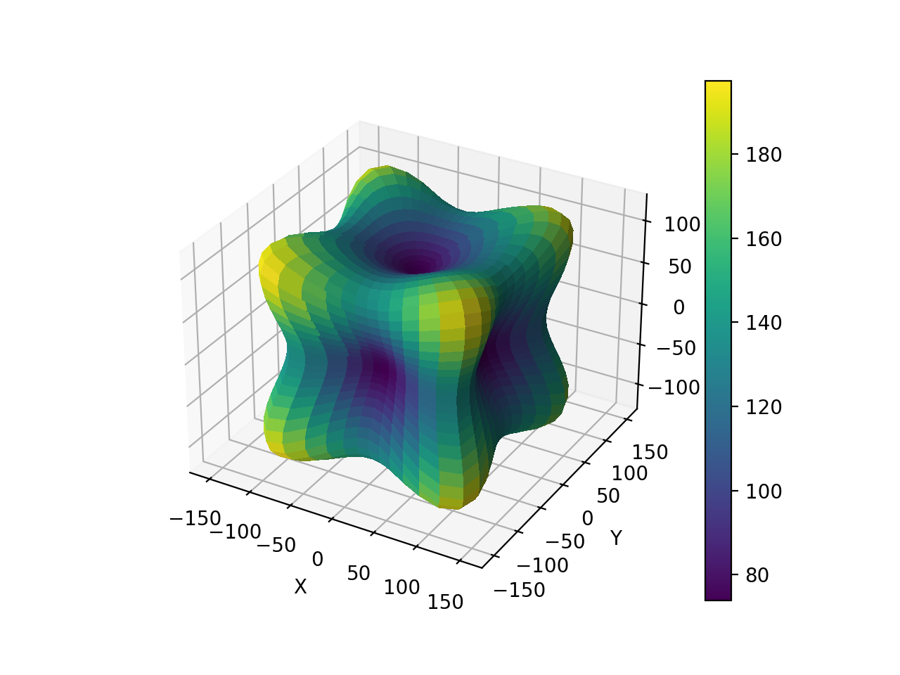
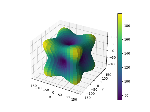
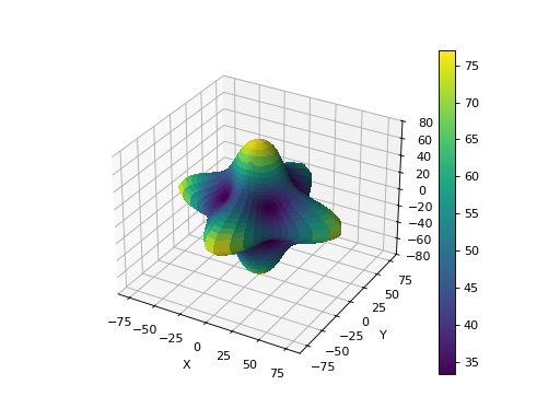
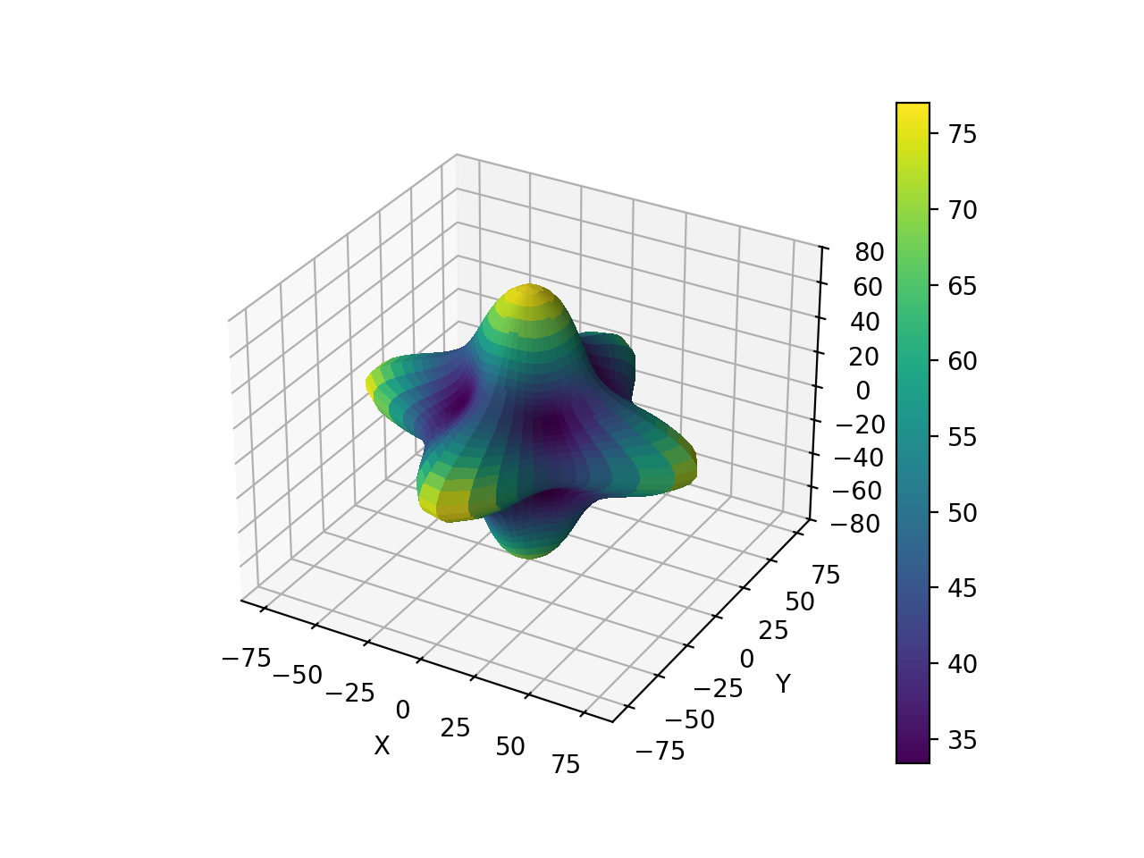
In order to fully evidence the directional dependence of the Young moduli, we can plot them as 3D surface:
from elasticipy.tensors.elasticity import StiffnessTensor
C = StiffnessTensor.cubic(C11=186, C12=134, C44=77)
E = C.Young_modulus
E.plot3D()
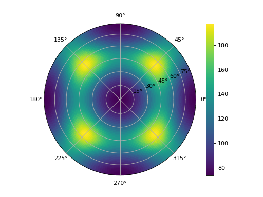
It is advised to use interactive plot to be able to zoom/rotate the surface. For flat images (i.e. to put in document/articles), we can plot the values as a Pole Figure (PF):
from elasticipy.tensors.elasticity import StiffnessTensor
C = StiffnessTensor.cubic(C11=186, C12=134, C44=77)
E = C.Young_modulus
E.plot_as_pole_figure()
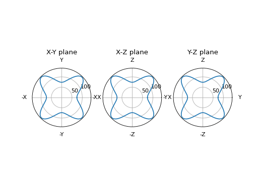
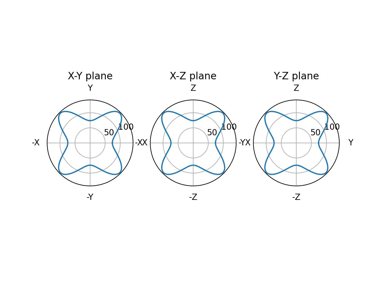
Alternatively, we can plot the Young moduli on X-Y, X-Z and Y-Z sections only:
from elasticipy.tensors.elasticity import StiffnessTensor
C = StiffnessTensor.cubic(C11=186, C12=134, C44=77)
E = C.Young_modulus
E.plot_xyz_sections()

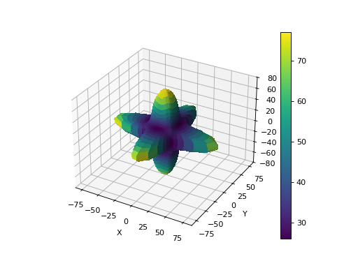
Hyperspherical functions
Hyperspherical functions cannot plotted as 3D surfaces, as their values depend on two orthogonal directions. But at least, for a each direction u, we can consider the mean value for all the orthogonal directions v when plotting:
from elasticipy.tensors.elasticity import StiffnessTensor
C = StiffnessTensor.cubic(C11=186, C12=134, C44=77)
G = C.shear_modulus
G.plot3D()

Instead of the mean value, we can consider other statistics, e.g.:
from elasticipy.tensors.elasticity import StiffnessTensor
C = StiffnessTensor.cubic(C11=186, C12=134, C44=77)
G = C.shear_modulus
G.plot3D(which='min')
This also works for max and std. These parameters also apply for pole figures (see above).
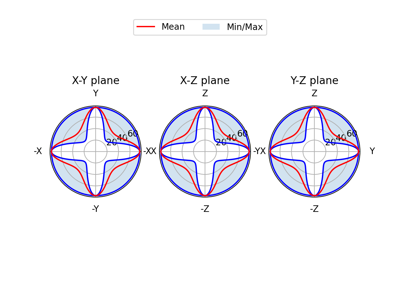
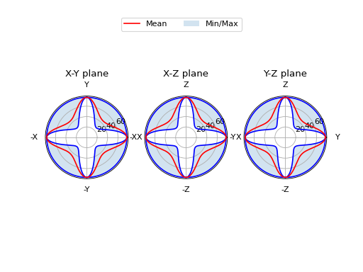
When plotting the X-Y, X-Z and Y-Z sections, the min, max and mean values are plotted at once:
from elasticipy.tensors.elasticity import StiffnessTensor
C = StiffnessTensor.cubic(C11=186, C12=134, C44=77)
G = C.shear_modulus
G.plot_xyz_sections()
Note
If you want to perform all the above tasks in a more interactive way, check out the GUI!
S. I. Ranganathan and M. Ostoja-Starzewski (2008), Universal Elastic Anisotropy Index, Phys. Rev. Lett., 101(5), 055504, . https://doi.org/10.1103/PhysRevLett.101.055504