Stress and strain tensors
This tutorial illustrates how we work on strain and stress tensors, and how Elasticipy handles arrays of tensors.
Single tensors
Let’s start with basic operations with the stress tensor. For instance, we can compute the von Mises and Tresca equivalent stresses:
>>> from elasticipy.tensors.stress_strain import StressTensor, StrainTensor
>>> stress = StressTensor.shear([1, 0, 0], [0, 1, 0], 1.0) # Unit XY shear stress
>>> print(stress.vonMises(), stress.Tresca())
1.7320508075688772 2.0
So now, let’s have a look on the strain tensor, and compute the principal strains and the volumetric change:
>>> strain = StrainTensor.shear([1,0,0], [0,1,0], 1e-3) # XY Shear strain with 1e-3 mag.
>>> print(strain.principal_strains())
[ 0.001  0.    -0.001]
>>> print(strain.volumetric_strain())
0.0
Linear elasticity
This section is dedicated to linear elasticity, hence introducing the fourth-order stiffness tensor. As an example, create a stiffness tensor corresponding to steel:
>>> from elasticipy.tensors.elasticity import StiffnessTensor
>>> C = StiffnessTensor.isotropic(E=210e3, nu=0.28)
>>> print(C)
Stiffness tensor (in Voigt mapping):
[[268465.90909091 104403.40909091 104403.40909091      0.
       0.              0.        ]
 [104403.40909091 268465.90909091 104403.40909091      0.
       0.              0.        ]
 [104403.40909091 104403.40909091 268465.90909091      0.
       0.              0.        ]
 [     0.              0.              0.          82031.25
       0.              0.        ]
 [     0.              0.              0.              0.
   82031.25            0.        ]
 [     0.              0.              0.              0.
       0.          82031.25      ]]
Considering the previous strain, evaluate the corresponding stress:
>>> sigma = C * strain
>>> print(sigma)
Stress tensor
[[  0.     164.0625   0.    ]
 [164.0625   0.       0.    ]
 [  0.       0.       0.    ]]
As an example, create a stiffness tensor corresponding to steel:
>>> from elasticipy.tensors.elasticity import StiffnessTensor
>>> C = StiffnessTensor.isotropic(E=210e3, nu=0.28)
>>> print(C)
Stiffness tensor (in Voigt mapping):
[[268465.90909091 104403.40909091 104403.40909091      0.
       0.              0.        ]
 [104403.40909091 268465.90909091 104403.40909091      0.
       0.              0.        ]
 [104403.40909091 104403.40909091 268465.90909091      0.
       0.              0.        ]
 [     0.              0.              0.          82031.25
       0.              0.        ]
 [     0.              0.              0.              0.
   82031.25            0.        ]
 [     0.              0.              0.              0.
       0.          82031.25      ]]
Considering the previous strain, evaluate the corresponding stress:
>>> sigma = C * strain
>>> print(sigma)
Stress tensor
[[  0.     164.0625   0.    ]
 [164.0625   0.       0.    ]
 [  0.       0.       0.    ]]
Note
As the components for the stiffness tensor were provided in MPa, the computed stress is given in MPa as well.
Conversely, one can compute the compliance tensor:
>>> S = C.inv()
>>> print(S)
Compliance tensor (in Voigt mapping):
[[ 4.76190476e-06 -1.33333333e-06 -1.33333333e-06  0.00000000e+00
   0.00000000e+00  0.00000000e+00]
 [-1.33333333e-06  4.76190476e-06 -1.33333333e-06  0.00000000e+00
   0.00000000e+00  0.00000000e+00]
 [-1.33333333e-06 -1.33333333e-06  4.76190476e-06  0.00000000e+00
   0.00000000e+00  0.00000000e+00]
 [ 0.00000000e+00  0.00000000e+00  0.00000000e+00  1.21904762e-05
   0.00000000e+00  0.00000000e+00]
 [ 0.00000000e+00  0.00000000e+00  0.00000000e+00  0.00000000e+00
   1.21904762e-05  0.00000000e+00]
 [ 0.00000000e+00  0.00000000e+00  0.00000000e+00  0.00000000e+00
   0.00000000e+00  1.21904762e-05]]
and check that we retrieve the correct (initial) strain:
>>> print(S * sigma)
Strain tensor
[[0.    0.001 0.   ]
 [0.001 0.    0.   ]
 [0.    0.    0.   ]]
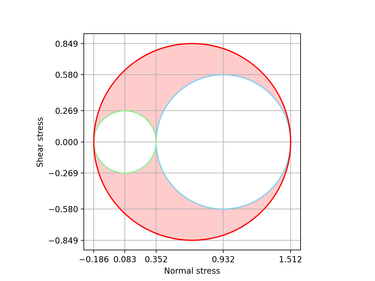
The Mohr circles
Let’s consider a random stress tensor:
>>> s = StressTensor.rand(seed=123) # Use seed to ensure reproducibility
>>> s
Stress tensor
[[0.68235186 0.11909641 0.57185244]
 [0.11909641 0.1759059  0.54433445]
 [0.57185244 0.54433445 0.81975456]]
A practical way to visualize its principal stresses and the possible shear stresses is to draw the Mohr circles:
from elasticipy.tensors.stress_strain import StressTensor
s = StressTensor.rand(seed=123) # Use seed to ensure reproducibility
fig, ax = s.draw_Mohr_circles()
fig.show()
In this figure, one can see that the principal stresses are around 1.512, 0.352 and -0.186 (in decreasing order); and that the maximum shear stress is around 0.849. Those can be checked by:
>>> s.principal_stresses()
array([ 1.51167769,  0.3519979 , -0.18566326])
>>> print(s.Tresca() / 2)
0.848670477704235
Note
As a recall, the Tresca’s equivalent stress is defined as twice the maximum shear stress.
Multidimensional tensor arrays
Elasticipy allows to process thousands of tensors at one, with the aid of tensor arrays. As an illustration, we consider the anisotropic behaviour of ferrite:
>>> C = StiffnessTensor.cubic(C11=274, C12=175, C44=89, phase_name='ferrite')
>>> print(C)
Stiffness tensor (in Voigt mapping):
[[274. 175. 175.   0.   0.   0.]
 [175. 274. 175.   0.   0.   0.]
 [175. 175. 274.   0.   0.   0.]
 [  0.   0.   0.  89.   0.   0.]
 [  0.   0.   0.   0.  89.   0.]
 [  0.   0.   0.   0.   0.  89.]]
Phase: ferrite
Let’s start by creating an array of 10 stresses:
>>> import numpy as np
>>> n_array = 10
>>> shear_stress = np.linspace(0, 100, n_array)
>>> sigma = StressTensor.shear([1,0,0],[0,1,0], shear_stress)  # Array of stresses corresponding to X-Y shear
>>> print(sigma[0])     # Check the initial value of the stress...
Stress tensor
[[0. 0. 0.]
 [0. 0. 0.]
 [0. 0. 0.]]
>>> print(sigma[-1])    # ...and the final value.
Stress tensor
[[  0. 100.   0.]
 [100.   0.   0.]
 [  0.   0.   0.]]
The corresponding strain array is evaluated with the same syntax as before:
>>> eps = C.inv() * sigma
>>> print(eps[0])     # Now check the initial value of strain...
Strain tensor
[[0. 0. 0.]
 [0. 0. 0.]
 [0. 0. 0.]]
>>> print(eps[-1])    # ...and the final value.
Strain tensor
[[0.         0.56179775 0.        ]
 [0.56179775 0.         0.        ]
 [0.         0.         0.        ]]
We can for instance compute the corresponding elastic energies:
>>> print(eps.elastic_energy(sigma))
[ 0.          0.69357747  2.77430989  6.24219725 11.09723956 17.33943682
 24.96878901 33.98529616 44.38895825 56.17977528]
Another application of working with an array of stress tensors is to check whether a tensor field complies with the
balance of linear momentum (see here
for details) or not. For instance, if we want to compute the divergence of sigma:
>>> sigma.div()
array([[ 0.        , 11.11111111,  0.        ],
       [ 0.        , 11.11111111,  0.        ],
       [ 0.        , 11.11111111,  0.        ],
       [ 0.        , 11.11111111,  0.        ],
       [ 0.        , 11.11111111,  0.        ],
       [ 0.        , 11.11111111,  0.        ],
       [ 0.        , 11.11111111,  0.        ],
       [ 0.        , 11.11111111,  0.        ],
       [ 0.        , 11.11111111,  0.        ],
       [ 0.        , 11.11111111,  0.        ]])
Here, the i-th row provides the divergence vector for the i-th stress tensor. See the full documentation for details about this function.
Apply rotations
Rotations can be applied on the tensors. If multiple rotations are applied at once, this results in tensor arrays.
Rotations are defined by scipy.transform.Rotation
(see here for details).
>>> from scipy.spatial.transform import Rotation
For example, let’s consider a random set of 1000 rotations:
>>> n_ori = 1000
>>> random_state = 1234 # This is just to ensure reproducibility
>>> rotations = Rotation.random(n_ori, random_state=random_state)
These rotations can be applied on the strain tensor
>>> eps_rotated = eps.rotate(rotations, mode='cross')
Option mode='cross' allows to compute all combinations of strains and rotation, resulting in a kind of 2D matrix of
strain tensors:
>>> print(eps_rotated.shape)
(10, 1000)
Therefore, we can compute the corresponding rotated stress array:
>>> sigma_rotated = C * eps_rotated
>>> print(sigma_rotated.shape)    # Check out the shape of the stresses
(10, 1000)
And get the stress back to the initial coordinate system:
>>> sigma = sigma_rotated * rotations.inv() # Go back to initial frame
As opposed to the rotate(..., mode='cross') (see above), we use * here to keep the same
dimensionality (perform element-wise multiplication). It is equivalent to:
>>> sigma = sigma_rotated.rotate(rotations.inv())
Finally, we can estimate the mean stresses among all the orientations:
>>> sigma_mean = sigma.mean(axis=1)     # Compute the mean over all orientations
>>> print(sigma_mean[-1]) # random
Stress tensor
[[ 5.35134832e-01  8.22419895e+01  2.02619662e-01]
 [ 8.22419895e+01 -4.88440590e-01 -1.52733598e-01]
 [ 2.02619662e-01 -1.52733598e-01 -4.66942413e-02]]
Actually, a more straightforward method is to define a set of rotated stiffness tensors, and compute their Reuss average:
>>> C_rotated = C * rotations
>>> C_Voigt = C_rotated.Voigt_average()
Which yields the same results in terms of stress:
>>> sigma_Voigt = C_Voigt * eps
>>> print(sigma_Voigt[-1])
Stress tensor
[[ 5.35134832e-01  8.22419895e+01  2.02619662e-01]
 [ 8.22419895e+01 -4.88440590e-01 -1.52733598e-01]
 [ 2.02619662e-01 -1.52733598e-01 -4.66942413e-02]]
See here for further details about the averaging methods.