Working with crystallographic textures
With the help of orix, Elasticipy allows to compute averages based on crystallographic texture (in addition to single orientations; see Finite number of orientations).
Define and compose textures
Discrete textures
A series of “usual” texture components (e.g. Goss, cube, Brass etc.) are already implemented in Elasticipy:
>>> from elasticipy.crystal_texture import DiscreteTexture
>>> goss = DiscreteTexture.Goss()
>>> goss
Crystallographic texture
φ1=0.00°, ϕ=45.00°, φ2=0.00°
This texture actually consists in a single orientation (as opposed to fibre textures, see below). It can be used to rotate a stiffness tensor as follows:
>>> from elasticipy.tensors.elasticity import StiffnessTensor
>>> C = StiffnessTensor.cubic(C11=186, C12=134, C44=77) # Copper, mp-30
>>> C * goss
Stiffness tensor (in Voigt mapping):
[[186. 134. 134.   0.   0.   0.]
 [134. 237.  83.   0.   0.   0.]
 [134.  83. 237.  -0.   0.   0.]
 [  0.   0.   0.  26.   0.   0.]
 [  0.   0.   0.   0.  77.   0.]
 [  0.   0.   0.   0.   0.  77.]]
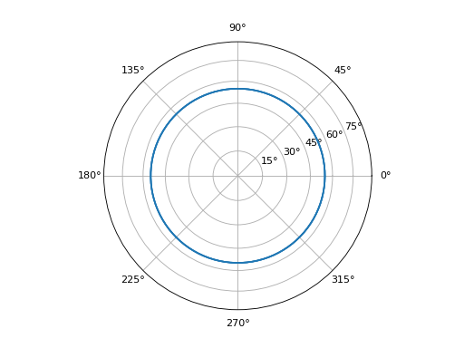
Fibre textures
Fibre textures are defined as uniformly distributed orientations around a given axis, leading to a single line when plotting an Orientation Distribution Function (ODF), hence the name. Therefore, there are three ways to define such textures.
The first one consists in defining the uvw direction to align with a given axis (related to the sample coordinate system). For instance, let’s consider the texture such that the <111> direction is aligned with the Z axis:
>>> from elasticipy.crystal_texture import FibreTexture
>>> from orix.crystal_map import Phase
>>> from orix.vector.miller import Miller
>>>
>>> phase = Phase(point_group='m-3m')   # Cubic symmetry
>>> m = Miller(uvw=[1,1,1], phase=phase)
>>> fibre_111 = FibreTexture.from_Miller_axis(m, [0,0,1])
>>> fibre_111
Fibre texture
<1. 1. 1.> || [0, 0, 1]
Actually, this texture is usually referred to as the γ fibre; therefore, a quicker way to define it is to use:
>>> gamma = FibreTexture.gamma()
This kind of shortcut also exists for alpha and epsilon textures (see here) for details).
The third way is to use two (out of the three) Bunge-Euler angles to define the fix angles (assuming that the orientations are uniformly distributed over the remaining angle). E.g.:
>>> fibre_phi2 = FibreTexture.from_Euler(phi1=0., Phi=0.)
>>> fibre_phi2
Fibre texture
φ1= 0.0°, ϕ= 0.0°
Then, the average stiffness resulting from such orientation distribution can be estimated from Voigt, Reuss or Hill method by integration over the all possible rotations. E.g.:
>>> Chill = C.Hill_average(orientations=fibre_phi2)
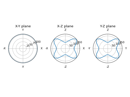
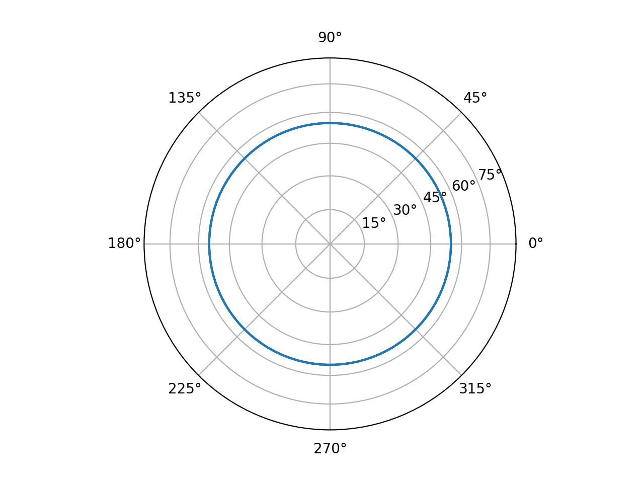
One can check that this results in a transversely isotropic behaviour by plotting the values of the Young modulus in planar sections. The full code is:
>>> from elasticipy.tensors.elasticity import StiffnessTensor
>>> from elasticipy.crystal_texture import FibreTexture
>>>
>>> C = StiffnessTensor.cubic(C11=186, C12=134, C44=77)
>>> fibre_phi2 = FibreTexture.from_Euler(phi1=0., Phi=0.)
>>> Chill = C.Hill_average(orientations=fibre_phi2)
>>> E = Chill.Young_modulus
>>> fig, ax = E.plot_xyz_sections()
>>> fig.show()
Composite textures
Different textures can be composed together to create a CompositeTexture object. For instance, if we consider a
a cubic material which exhibits 40% of uniform texture, 30% of <111>||[0,0,1] and balanced copper texture, we can do the
following:
>>> from elasticipy.crystal_texture import UniformTexture
>>> t = 0.4 * UniformTexture() + 0.3 * fibre_111 +  0.3 * DiscreteTexture.copper()
>>> t
Mixture of crystallographic textures
 Wgt.  Type      Component
 ------------------------------------------------------------
 0.40  uniform   Uniform distribution over SO(3)
 0.30  fibre     <1. 1. 1.> || [0, 0, 1]
 0.30  discrete  φ1=90.00°, ϕ=35.26°, φ2=45.00°
Again, the Hill average can be computed as follows:
>>> C.Hill_average(orientations=t)
Stiffness tensor (in Voigt mapping):
[[229.93 115.   109.07   0.     0.17  -0.  ]
 [115.   224.47 114.53  -0.     6.03   0.  ]
 [109.07 114.53 230.4   -0.    -6.2   -0.  ]
 [  0.    -0.    -0.    38.57  -0.     5.34]
 [  0.17   6.03  -6.2   -0.    35.04  -0.  ]
 [  0.     0.    -0.     5.34   0.    38.52]]
Random sampling
Sample of orientations can be drawn from all kind of textures. While a “random” sample from a single discrete texture does not make any sense, it can be of great interest for fibres or composite textures.
For instance, a sample of 10 orientations can be drawn from the composite texture defined above as follows:
>>> sample = t.sample(num=10, seed=123) # Seed here is used to ensure reproducibility
>>> sample
Orientation (10,) 1
[[ 0.1157  0.5901  0.2194 -0.7683]
 [ 0.3954 -0.6714 -0.421   0.4644]
 [ 0.9571 -0.1986 -0.2022  0.0609]
 [ 0.0802 -0.7012  0.3947 -0.5883]
 [ 0.1952 -0.8854  0.3814  0.1802]
 [-0.4814  0.4494  0.097   0.7463]
 [ 0.3647 -0.2798 -0.1159 -0.8805]
 [ 0.3647 -0.2798 -0.1159 -0.8805]
 [ 0.3647 -0.2798 -0.1159 -0.8805]
 [ 0.3647 -0.2798 -0.1159 -0.8805]]
One may note that here, the 4 last orientations are the same. This is because it relates to the copper texture:
>>> DiscreteTexture.copper().orientation
Orientation (1,) 1
[[ 0.3647 -0.2798 -0.1159 -0.8805]]
Plotting
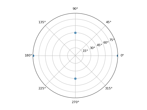
Pole figures can be drawn to evidence how each texture works. For instance, the (pure) Goss texture results in the following pole figure:
>>> from elasticipy.crystal_texture import DiscreteTexture
>>> Goss = DiscreteTexture.Goss()
>>> fig, ax = Goss.plot_as_pole_figure(uvw=[1,0,0], symmetrise=True)
>>> fig.show()

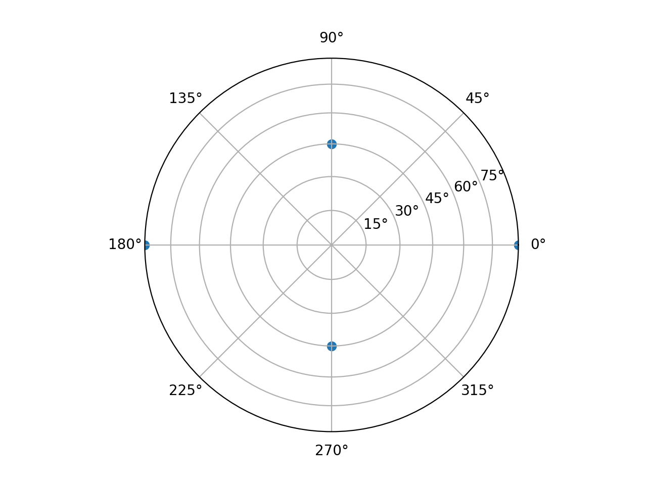
Fibre textures can be drawn in a simular way. E.g.:
>>> from elasticipy.crystal_texture import FibreTexture
>>>
>>> gamma = FibreTexture.gamma()
>>> fig, ax = gamma.plot_as_pole_figure(uvw=[1,0,0], symmetrise=True)
>>> fig.show()
