Computing and plotting engineering constants

This page illustrates how one can create stiffness (or compliance) tensors, manipulate them and plot some elasticity-related values (e.g. Young modulus).

Direction-dependent Young moduli

First, create a stiffness tensor with a given symmetry (let say, monoclinic):

>>> from Elasticipy.FourthOrderTensor import StiffnessTensor
>>> C = StiffnessTensor.monoclinic(phase_name='TiNi',
...                                C11=231, C12=127, C13=104,
...                                C22=240, C23=131, C33=175,
...                                C44=81, C55=11, C66=85,
...                                C15=-18, C25=1, C35=-3, C46=3)

Let’s investigate the Young modulus:

>>> E = C.Young_modulus

Here E is a SphericalFunction object. It means that its value depends on the considered direction. For instance, let’s see its value along the x, y and z directions:

>>> Ex = E.eval([1,0,0])
>>> Ey = E.eval([0,1,0])
>>> Ez = E.eval([0,0,1])
>>> print((Ex, Ey, Ez))
(124.52232440357189, 120.92120854784433, 96.13750721721384)

Actually, a more compact syntax, and a faster way to do that, is to use:

>>> import numpy as np
>>> print(E.eval(np.eye(3)))
[124.5223244  120.92120855  96.13750722]

To quickly see the min/max value of a SphericalFunction, just print it:

>>> print(E)
Spherical function
Min=26.283577707639264, Max=191.396591469876

It is clear that this material is highly anisotropic. This can be evidenced by comparing the mean and the standard deviation of the Young modulus:

>>> E_mean = E.mean()
>>> E_std = E.std()
>>> print(E_std / E_mean)
0.45580071168605646

Another way to evidence anisotropy is to use the universal anisotropy factor [1]:

>>> C.universal_anisotropy
5.1410095516414085

Shear moduli and Poisson ratios

The shear modulus can be computed from the stiffness tensor as well:

>>> G = C.shear_modulus
>>> print(G)
Hyperspherical function
Min=8.748742560860673, Max=86.60555127546397

Here, the shear modulus is a HyperSphericalFunction object because its value depends on two orthogonal directions (in other words, its arguments must lie on an unit hypersphere S3).

Let’s compute its value with respect to X and Y directions:

>>> print(G.eval([1,0,0], [0,1,0]))
84.88888888888889

The previous consideration also apply for the Poisson ratio:

>>> print(C.Poisson_ratio)
Hyperspherical function
Min=-0.5501886056193359, Max=1.4394343811865082

Plotting

Spherical functions

In order to fully evidence the directional dependence of the Young moduli, we can plot them as 3D surface:

>>> E.plot3D()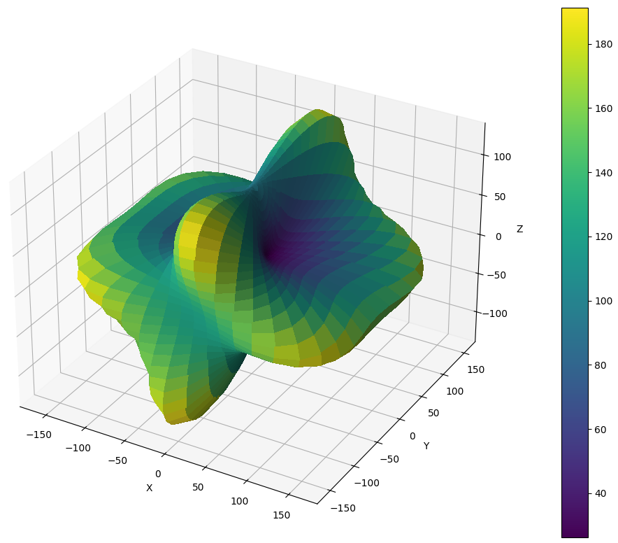

It is advised to use interactive plot to be able to zoom/rotate the surface. For flat images (i.e. to put in document/articles), we can plot the values as a Pole Figure (PF):

>>> E.plot_as_pole_figure()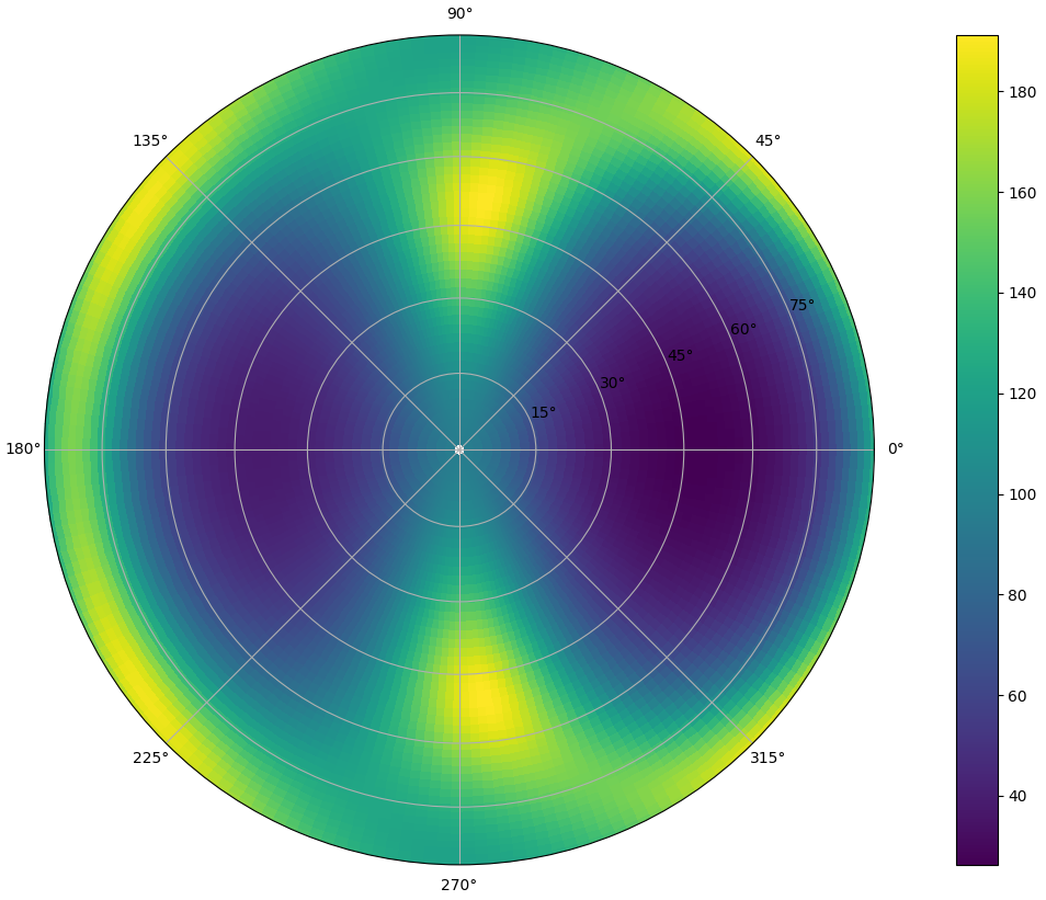

Alternatively, we can plot the Young moduli on X-Y, X-Z and Y-Z sections only:

>>> E.plot_xyz_sections()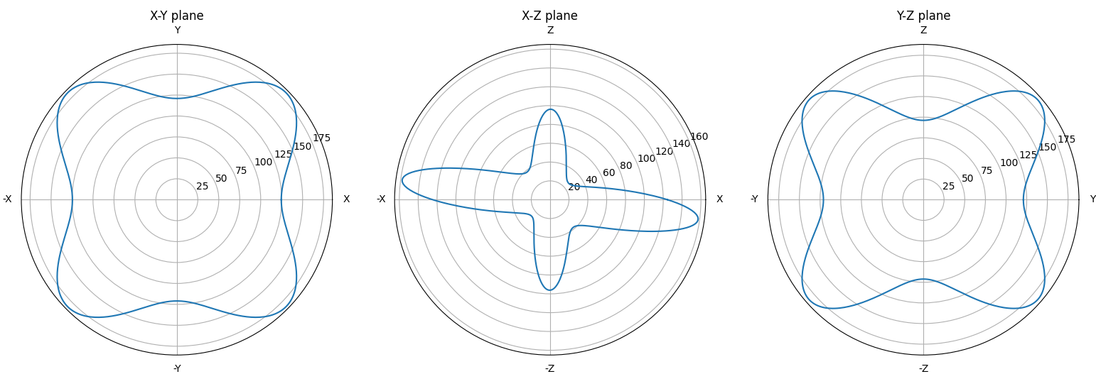

Hyperspherical functions

Hyperspherical functions cannot plotted as 3D surfaces, as their values depend on two orthogonal directions. But at least, for a each direction u, we can consider the mean value for all the orthogonal directions v when plotting:

>>> G.plot3D()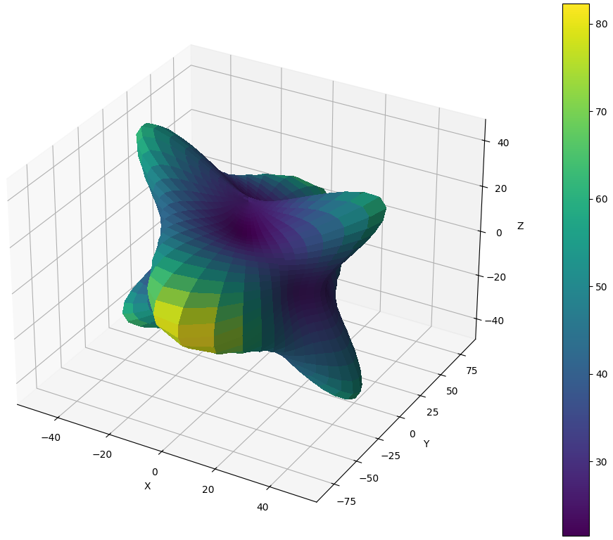

Instead of the mean value, we can consider other statistics, e.g.:

>>> G.plot3D(which='min')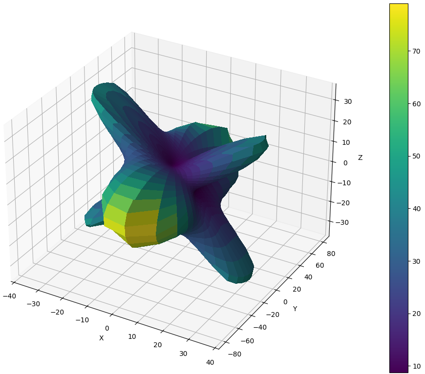

This also works for max and std. These parameters also apply for pole figures (see above).

When plotting the X-Y, X-Z and Y-Z sections, the min, max and mean values are plotted at once:

>>> G.plot_xyz_sections()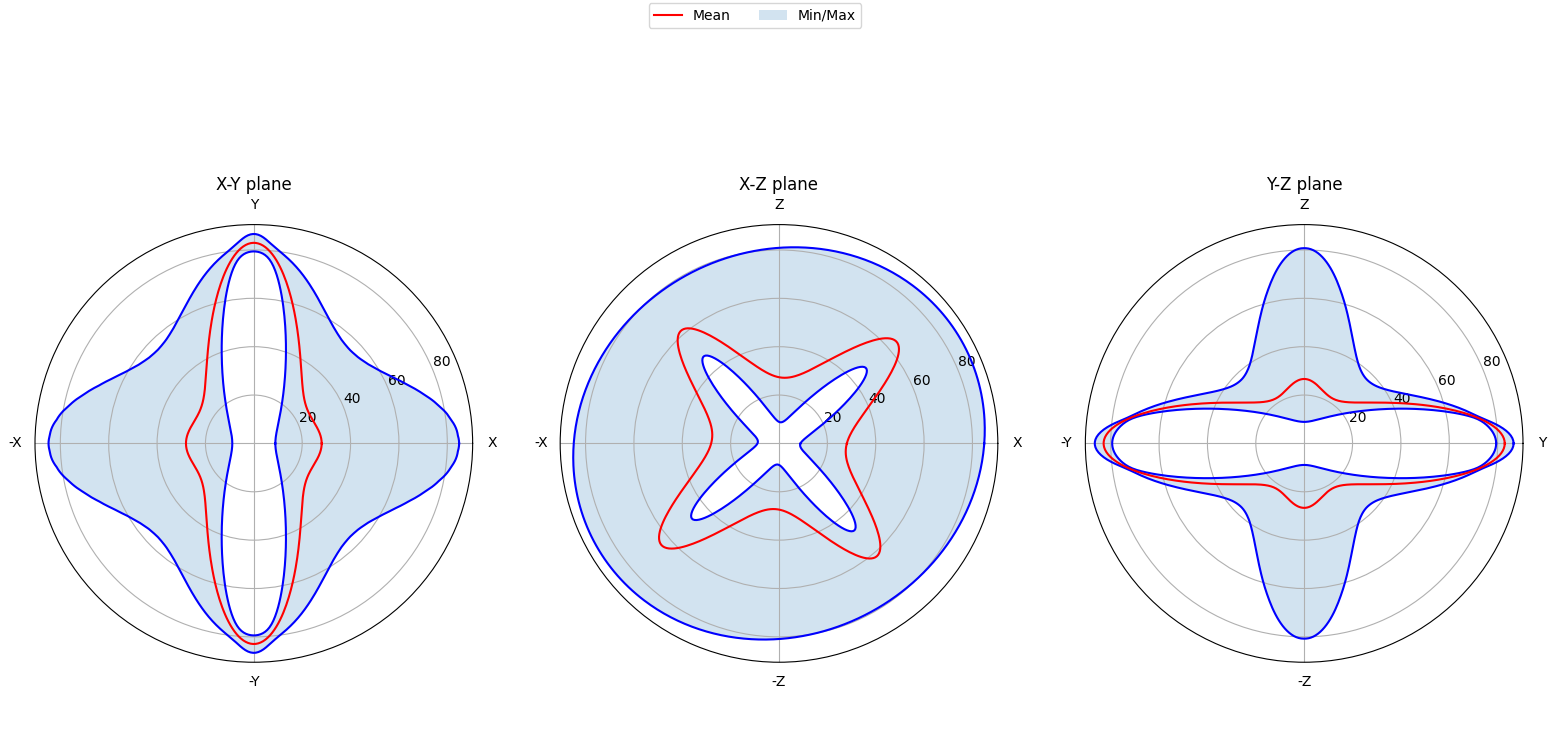

Note

If you want to perform all the above tasks in a more interactive way, check out the GUI!