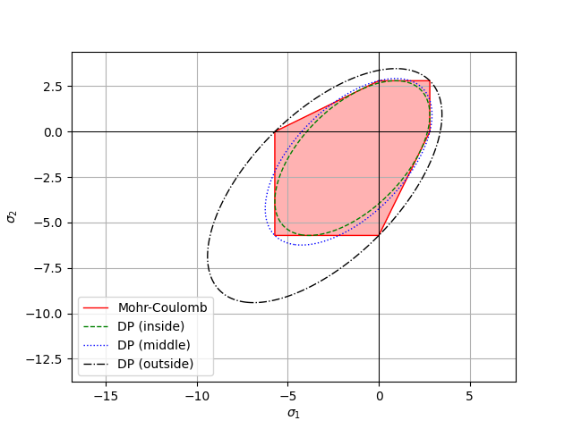
Plot in 2D the Mohr-Coulomb and Drucker-Prager yield surface

The example illustrates in 2D the differences between the Mohr-Coulomb and the Drucker-Prager yield criteria.

from elasticipy.yield_criteria import DruckerPrager, MohrCoulomb
c   = 2
phi = -20
mc = MohrCoulomb(c, phi)

When expressed in terms of cohesion (c) and friction angle (phi), there are three ways to ‘fit’ the Drucker-Prager (DP) yield criterion with that of Mohr-Coulomb (see here):

pg1 = DruckerPrager.from_cohesion_friction_angle(c, phi, fit='inside')
pg2 = DruckerPrager.from_cohesion_friction_angle(c, phi, fit='middle')
pg3 = DruckerPrager.from_cohesion_friction_angle(c, phi, fit='outside')

fig, ax = mc.plot2D()
fig, ax = pg1.plot2D(fig=fig, ax=ax, label='DP (inside)', color='green', alpha=0., linestyle='dashed')
fig, ax = pg2.plot2D(fig=fig, ax=ax, label='DP (middle)', color='blue', alpha=0., linestyle='dotted')
fig, ax = pg3.plot2D(fig=fig, ax=ax, label='DP (outside)', color='black', alpha=0., linestyle='dashdot')
ax.legend()
fig.show()