Compute and plot wave velocities

This example shows how to compute the wave velocities from the stiffness tensor, and how to plot them

Define the stiffness tensor for forsterite

We define the stiffness tensor for a forsterite (taken from the similar tutorial for MTEX users.) as well as the mass density

from elasticipy.tensors.elasticity import StiffnessTensor
C = StiffnessTensor.orthorhombic(phase_name='forsterite',
                                 C11=320, C12=68.2, C13=71.6, C22=196.5, C23=76.8,
                                 C33=233.5, C44=64, C55=77, C66=78.7)
rho = 3.36 # kg/dm³!
print(C)

Stiffness tensor (in Voigt mapping):
[[320.   68.2  71.6   0.    0.    0. ]
 [ 68.2 196.5  76.8   0.    0.    0. ]
 [ 71.6  76.8 233.5   0.    0.    0. ]
 [  0.    0.    0.   64.    0.    0. ]
 [  0.    0.    0.    0.   77.    0. ]
 [  0.    0.    0.    0.    0.   78.7]]
Phase: forsterite

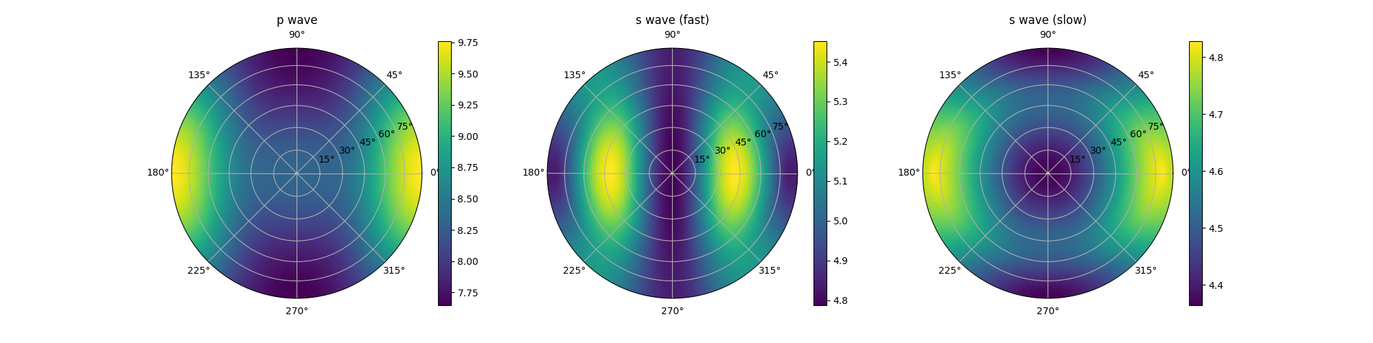
Compute the velocities of primary and secondary waves

cp, cs_fast, cs_slow = C.wave_velocity(rho)

Plot them as three independent pole figures:

import matplotlib.pyplot as plt
fig = plt.figure(figsize=(20, 5))
cp.plot_as_pole_figure(subplot_args=(131,), title='p wave', fig=fig)
cs_fast.plot_as_pole_figure(subplot_args=(132,), title='s wave (fast)', fig=fig)
cs_slow.plot_as_pole_figure(subplot_args=(133,), title='s wave (slow)', fig=fig)

(<Figure size 2000x500 with 6 Axes>, <PolarAxes: title={'center': 's wave (slow)'}>)